A Hybrid Approach for Android Malicious Software Classification
Abstract
Android operating systems have grown in popularity and are currently being increasingly used on smartphone devices. Because of the quickly expanding quantity of Android malware and the potential safeguard of vast amounts of data kept on Android devices, the identification and categorization of Android malware is regarded as a big data challenge. Researchers started using deep learning (DL) techniques for malware detection, according to the most recent state-of-the-art studies. Nevertheless, researchers and practitioners face challenges such as the choice of DL architecture, extracting and processing features and evaluating results. In this paper, several traditional and hybrid machine learning (ML) models were developed and analyzed in detail to classify Android malware. First, some state-of-the-art DL model has been developed like multi-layer perceptron (MLP), deep neural network (DNN), recurrent neural network (RNN), long short-term memory (LSTM), convolutional neural network (CNN) and later several hybrid models have been developed by combining DNNs with support vector machine (SVM). Second, we have focused on maximizing achievement by fine-tuning a variety of configurations to guarantee the best possible combination of the hyper-parameters and attain the maximum statistical metric value. Finally, we have accomplished performance analysis between these hybrid models and a model based on VGG-16-CNN-1D along with SVM has been proposed to enhance the accuracy and efficacy of large-scale Android malware detection which outperforms all the other developed models using Drebin Dataset. Among the DL methods, DNN achieved the highest F1 score 99.07%. After doing a comparison between hybrid models, it was found that DNN-SVM achieved 99.12% while VGG16-CNN-1D-SVM achieved 98.56% precision, 98.78% recall and 99.20% F1 score, respectively.
1. Introduction
Android has quickly become the fastest-growing mobile operating system (OS), thanks to contributions from the open-source Linux community, as well as the availability of software, hardware and carrier partners. The open-source nature of Android, as well as third-party distribution centers, a robust SDK and Java’s ubiquity as a programming language, have all contributed to its growth. According to Statcounter1 in September 2022, Android has a global market share of 71.62% among mobile OSs followed by Apple iOS 27.73%. Android is the mobile platform that has been attacked the most by malware that aims to steal personal information or control the user’s devices due to its open environment. Furthermore, Android features several third-party application shops, making it simple for fraudsters to repackage Android apps with harmful code. The detection approaches for Android malware can be split into static analysis, dynamic analysis and hybrid analysis methods based on diverse analysis methods.2 Static analysis extracts identical static features (such as Java code, permissions, network addresses, intent filters, hardware components, strings, etc.) from the Java bytecode or manifest file without executing the code, whereas virtual machines and sandboxes are used to execute applications in isolated settings in dynamic analysis. The behavior of the program can be studied as it is being executed. Hybrid analysis is an approach that combines static and dynamic analysis approaches. It’s designed to examine malware from a variety of perspectives, and it’s thought to be a superior approach to the individual analysis approaches.
Recent research has presented machine learning (ML)-based malware detection systems for their ability to detect and classify Android malware. Traditional ML has proven to be extremely effective at detecting Android malware using hand-crafted features. However, the feature engineering method is error-prone and time-consuming3 and most ML-based approaches necessitate security specialists manually defining the attributes that characterize Android malware, which strongly relies on experts’ expertise, level of competence and subject knowledge.4 As a result, there is a need for robust detection systems in Android that can protect against continually emerging threats.
To overcome the challenges of feature engineering, researchers are using deep learning (DL) techniques that allow features to be learned instinctively5 and at several levels of abstraction, improving generalizability and relieving security specialists of time-consuming and potentially error-prone feature engineering activities.6 DL methods outperform traditional ML methods in detecting malware on Android.7 The technique for detecting Android malware is continually being enhanced and innovated by researchers. We have tried to present a thorough analysis of the most cutting-edge technology available today which is summarized in this section.
As an experimental strategy while using conventional ML methods, Kapratwar et al.8 suggested reverse engineering and the outcome showed a 96.6% detection rate when the random forest (RF) method was utilized, with a marginal difference of 0.069% from the worst detection technique. Zhu et al.9 proposed a low-cost and highly effective way to extract static features as essential aspects and use the ensemble Rotation Forest and the conclusions demonstrate that the suggested strategy achieves a high accuracy of 88.26% with 88.40% sensitivity at 88.16% precision. Salehi and Amini10 used the dynamic detection strategy on two malware datasets separately, and utilizing the ServiceMonitor approach, the RF classifier accurately identified the malware with 96% accuracy. An innovative Android malware detection method that uses a deep convolutional neural network (CNN) and malware categorization based on static analysis of the raw opcode sequence from a disassembled program was proposed by McLaughlin et al.11 Islam et al.12 conducted a thorough analysis to assess the efficacy of stacking generalization in N-gram techniques. In comparison to bigram and trigram, it has been discovered that unigram gives more than 97% accuracy when stacking.
In addition, Kim et al.13 proposed a multimodal DL method that makes use of a variety of features to reflect the characteristics of Android applications from a variety of perspectives and utilizing the feature extraction model, it was possible to maximize the advantages of incorporating variety of feature types. Damodaran et al.14 trained Hidden Markov Models (HMMs) on static and dynamic feature sets and assessed the resulting detection rates over many different malware families and in their studies, they found that a fully dynamic approach often produces the best detection rates. Besides, Costa and Aria15 suggested an emulation-based method in sandbox systems that could detect malware with privilege escalation and zero-day vulnerabilities but some malware, nevertheless, is aware of the virtual nature of the environment and tends to avoid detection. Lakshmanarao and Shashi16 devised a CNN architecture for DL that converts malicious and benign Android APKs into images based on their sizes. Using little information required, the suggested DL system with CNN may reach 97.76% accuracy. Singh et al.17 proposed a fine-tuned CNN that is applied which turns the malware’s non-intuitive attributes into fingerprint images and while evaluating gray-scale malware images, the softmax layer of CNN was replaced with ML techniques such as RF, K-nearest neighbor (KNN) and support vector machine (SVM) which can achieve an accuracy of 92.59%. A new Android malware detection model built on a temporal convolution network (TCN) is proposed by Zhang et al.18 First, four gray-scale image datasets with four distinct combinations of texture features were constructed by merging XML files and DEX files, and experimental results demonstrate that adding XML files is helpful for Android malware identification. Wang et al.19 suggested a hybrid model that combines CNN and deep autoencoder (DAE), with CNN-S model accuracy being 5% higher than SVM accuracy. When compared to CNN-S, the DAE-CNN requires 83% less training time.
Dina et al.20 used a CNN to train a detection model and apply it to categorize malware that is effective in detecting malware encrypted using polymorphic techniques. They directly extracted the bytecode file from the Android APK file and converted the bytecode file into a two-dimensional bytecode matrix. Besides, to extract comprehensive features from Android applications and construct an autonomous detection engine, DeepDetector, to identify malicious applications, Li et al.21 offered a novel technique. Alzaylaee et al.22 also suggested utilizing DL-Droid to detect malicious Android applications through dynamic analysis and stateful input generation. As DL-Droid is demonstrated to be superior to the current state-of-the-art systems using state-based input generation. Jiang et al.23 developed a prototype known as AOMDroid after proposing a successful method based on the TFIDF algorithm to recognize different opcode sequences and they use transfer learning to accomplish the goals. A long short-term memory (LSTM)-based model24 was created using benign and malware samples that were investigated using both static and dynamic analysis techniques, and it achieved a classification accuracy of 99.94% when tested on augmented samples and 86.5% when tested on real data with samples of newly emerged malware. PetaDroid, a framework for precise Android malware detection introduced by Karbab and Debbabi20 uses unique methodologies built on top of ML and natural language processing (NLP) methods to enable adaptive, accurate and resilient detection and family grouping. PetaDroid performs better than other cutting-edge systems like MalDozer, DroidAPIMiner and MaMaDroid. Nath et al.25 proposed a static-based analysis technique that uses boosting algorithms to determine the relative importance of developing ML Models using a reduced set of features and the results of this study presented that, among the category of boosting algorithms, CatBoost and GradientBoost had the highest F1 score (93.9%).
ESDroid, a new event-aware dynamic slicing technique for streamlining inputs for Android apps, is presented by Win et al.26 and it was tested using 38 real-world apps against AndroidSlicer and 10 apps against Mandoline and by removing unnecessary nodes, the findings demonstrate that ESDroid performs better than AndroidSlicer and Mandoline. In order to reduce label errors in datasets containing Android malware, Wang et al.27 proposed an efficient method called MalWhiteout. They do this by introducing Confident Learning (CL), a sophisticated approach for estimating noise, to the field of Android malware detection. Experiments demonstrate that MalWhiteout is capable of detecting label noises with over 94% accuracy even at a high noise ratio (i.e., 30%) of the dataset. Zhang et al.28 introduced Andre, a new ANDroid Hybrid REpresentation learning approach to clustering Android malware with inaccurate labeling and it preserves heterogeneous information from various sources, such as static code analysis results, app meta-information and raw AV vendor labels, to jointly learn a hybrid representation.
The objectives of this research are, firstly, to build several hybrid models by combining deep neural networks (DNNs) with classical ML algorithms. Then, we have also put up the novel idea of customizing VGG-like model for one-dimensional (1D) convolution and accomplished the performance analysis between those hybrid models. Finally, to propose an efficient technique for the detection of Android malware through hybrid approaches using static features regarding the Drebin Dataset. As a result, this research will identify the shortcomings of the current methods and provide prospective directions for further research.
The formation of this paper is as follows. Section 2 discusses the overall research methodology, while the experimental results, analysis and discussions are described in Sec. 3. Finally, conclusion and future research are narrated in Sec. 4.
2. Methodology
This section briefly depicts the study’s methodological overview. A brief overview of the research methodology is shown in Fig. 1 which includes data acquisition, data pre-processing, model selection, model configuration set up and model definition, model training and hyper-parameter tuning, performance evaluation and result analysis. The stages are briefly discussed in the following sections.
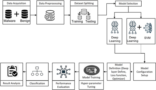
Fig. 1. Model architecture of android malware detection study.
2.1. Data acquisition
The dataset used in the experiment is from the University of Gottingen’s Drebin project.29 Drebin samples are broadly used in the scientific community. A total of 215 features were obtained from 15,036 applications in this dataset (9476 benign and 5560 malware). This dataset was also employed to create and assess a multilevel classifier fusion method for identifying Android malware.30 Dataset feature categories are shown in Fig. 2.
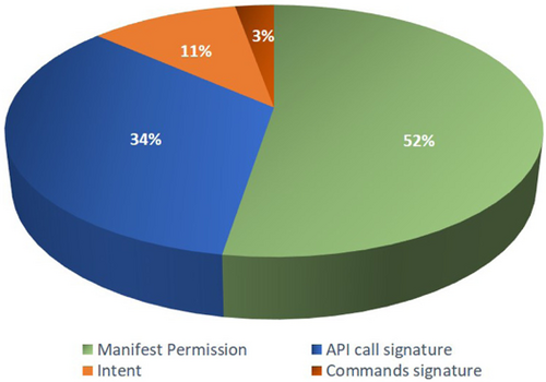
Fig. 2. Dataset feature categories.
2.2. Data pre-processing and splitting
During this phase, the dataset is first subjected to label encoding to convert the labels into a machine-readable numeric form (“0”, “1”). It is an essential pre-processing step in the structured dataset’s supervised learning process. Second, special characters in the dataset include “?” and “S” which have been removed by using dropna from rows and columns after setting them to NaN. Third, the target feature was encoded as it was labeled as “S”, short for malware and “B”, short for Benign. A random train–test split of 80:20 was applied to the dataset, where 80% data were considered as the train set while 20% data was considered as the test set. Final categorical features have been pre-processed using one hot encoding to supply them to the VGG neural network, which in turn enhances the predictions and classification accuracy of a model.
2.3. Hybrid model development
In this step, different DL algorithms are chosen based on the recent works relating to Android malware classification, which included multi-layer perceptron (MLP), DNN, recurrent neural network (RNN), LSTM, CNN, VGG-16 and VGG-19. As per the objectives of this study, SVM is selected to build a hybrid model along with state-of-the-art DL models. After extracting features from DL techniques, SVM is pushed between dense layers for controlling loss function and getting better classification performance. Each of the algorithms and their working procedure is analyzed in detail in the following sections.
2.3.1. Architecture of MLP with SVM
MLP is defined by many layers of input nodes coupled as a directed graph between the input and output layers, which are used for supervised learning format and use back propagation to train the network.31 In this hybrid model approach, SVM has been added with MLP before the last dense layer. Figure 3 shows the model architecture. The input layer is shaped with 215 neurons and a total of 46,440 parameters. Two dense layers with 100 and 40 neurons, respectively, have been designed where the second dense layer adopts a softmax activation function to normalize the output of a network to a probability distribution over the predicted output class. Later, the normalized output has been passed to the output layer with 01 neuron.
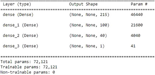
Fig. 3. MLP-SVM model architecture.
Epoch versus loss: Train and validation loss showed a higher value at the beginning and started to decrease while the epoch is increasing. Figure 4 shows the graph where some drastic changes have been shown in the validation loss and around 170 epoch dramatic changes have been shown. Validation has been done smoothly for the MLP-SVM hybrid model because the model is regularizing within a short period of time as data are randomly shuffled.
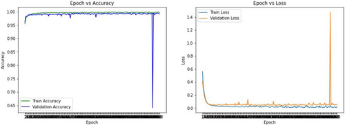
Fig. 4. MLP-SVM model validation.
2.3.2. Architecture of DNN with SVM
DNNs are multilayer variations of conventional artificial neural networks (ANNs), and they have lately gained popularity due to their improved ability to learn both the underlying structure of the input data vectors and the nonlinear input-output mapping.32 In this hybrid model approach, SVM has been added with DNN. Figure 5 shows the model architecture. The input layer is shaped with 215 neurons and a total of 46,440 parameters. Five dense layers are designed with neurons in decreasing order to minimize the features and last of all fit into the output layer. The last two-dense layer consists of 40 neurons and the output layer has 41 parameters. Here, relu activation function has been employed in dense layers to achieve a nonlinear transformation of the data and sigmoid has been utilized in the output layer to forecast the probability as an output.
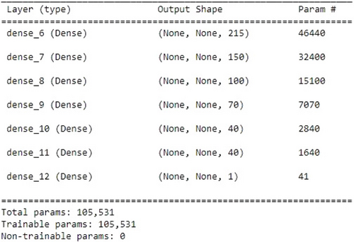
Fig. 5. DNN-SVM model architecture.
Epoch versus accuracy: While the epoch is increasing the train and validation accuracy is also increasing in parallel. Around 156 epoch validation accuracy falls to a dramatic level. Some significant spikes were also shown at the end of the training process.
Epoch versus loss: Figure 6 shows the train and validation loss. From the beginning, the loss has been fluctuating at a notable level and it is trying to reach saturation level. Around 150 epochs, a drastic change has been shown and as data were randomly shuffled, it regularizes the outcome.
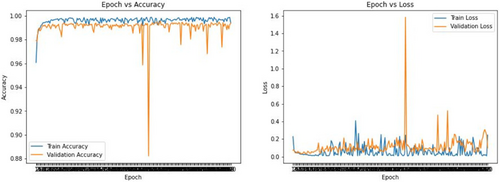
Fig. 6. DNN-SVM model validation.
2.3.3. Architecture of RNN with SVM
RNNs are a type of neural network where the output from one phase is used as the input for the following one.33 Since RNNs achieve the same results by carrying out the same task on all inputs or hidden layers, they use the same parameters for each input and have a “memory” that holds all information about the calculations. In this hybrid model approach, SVM has been added with RNN. Figure 7 shows the model architecture. The input layer is shaped with 215 neurons and a total of 31,600 parameters. One dense layer is designed with 100 neurons and the output layer contains 101 parameters. As the RNN model is simple in architecture, one dense layer and a linear activation function have been chosen here.
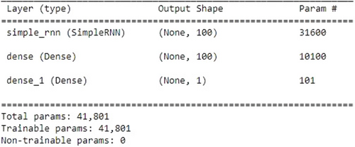
Fig. 7. RNN-SVM model architecture.
Epoch versus accuracy: Figure 8 shows that train accuracy was less at the beginning, and it tries to increase while the validation also increases. Train accuracy outruns the validation which indicates the train was inconsistent in this hybrid model.
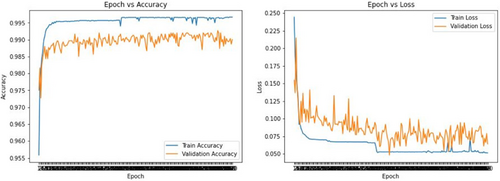
Fig. 8. RNN-SVM model validation.
Epoch versus loss: Train and validation loss showed a higher value at the beginning and started to decrease while the epoch was increasing. Figure 8 shows significant changes in validation loss and train loss showing inconsistent results. Around 93 epochs, it tries to be saturated.
2.3.4. Architecture of LSTM with SVM
LSTMs, a type of RNN whose default function is to recall past information over long periods of time, can be used to learn and remember long-term dependencies.34 Data are tracked over time via LSTMs. They are useful in time-series prediction because they retain memories of previous inputs. In this hybrid model approach, SVM has been added with LSTM. Figure 9 shows the model architecture. The input layer is shaped with 215 neurons and a total of 126,400 parameters. Parameters are reduced to 7880 using a dense layer followed by another LSTM layer. The output layer contains 41 parameters and uses a sigmoid function which has a gradient that rapidly converges towards 0. It makes the model slow in the training process thus, a learning rate of 0.01 has been maintained.
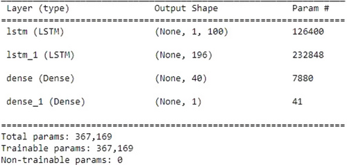
Fig. 9. LSTM-SVM model architecture.
Epoch versus accuracy: Figure 10 shows that train accuracy was less at the beginning, and it tries to increase while the validation also increases. There was a significant gap between the train and validation loss. Though two lines are saturated around 90 epochs, it shows inconsistent training.
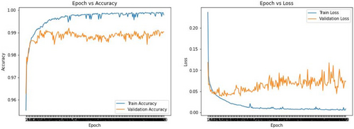
Fig. 10. LSTM-SVM model validation.
Epoch versus loss: Train and validation loss showed a higher value at the beginning and started to decrease while the epoch was increasing. Figure 10 shows significant changes in validation.
2.3.5. Architecture of CNN-1D with SVM
CNN35 is a DL system that can take an input image and give different aspects and objects in the image learnable weights and biases to enable them to be distinguished. Convolutional, pooling and fully connected (FC) layers are the three types of layers that make up a CNN. If adequate training data is available, CNN has a deep structure and can automatically learn several layers of malware feature representations. In this hybrid model approach, SVM has been added with Conv1D. Figure 11 shows the model architecture. The input layer is shaped with 215 neurons and a total of 256 parameters. The maxpooling layer has been used to reduce the number of neurons. Initially, 64 filter sizes and 03 strides have been used. After flattening and dense layers, the SVM has been pushed to get better classification accuracy. At the output layer, sigmoid is used to predict the probability as a classification output.
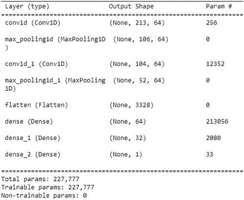
Fig. 11. Conv1D-SVM model architecture.
In Fig. 12, train and loss validation has been shown where the epoch increases and accuracy tends to decrease and shows some significant spikes. Accuracy shows around 99% of value where it goes to saturation after a few epochs. Loss for training and validation decreases gradually and at some point, validation loss deviates and increases. Around 145 epochs, it has been saturated and suddenly becomes low around 186 epochs.
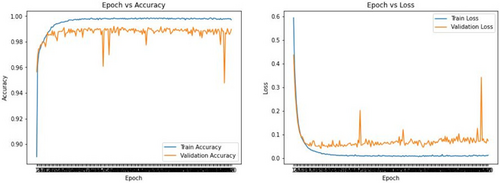
Fig. 12. Conv1D-SVM model validation.
2.3.6. Architecture of VGG-16-Conv1D with SVM
VGG-16 was proposed by Simonyan and Zisserman of the visual geometry group lab of Oxford University in 2014 in the paper “Very deep convolutional networks for large-scale image recognition”.36 The number 16 in VGG-16 stands for 16 weighted layers. Thirteen convolutional layers, five maxpooling layers, three dense layers, and a total of 21 layers make up VGG-16, but only sixteen of them are weight layers, also known as learnable parameters layers. The most distinctive feature of VGG-16 is that it prioritized having convolution layers of 3×3 filters with a stride 1 and always utilized the same padding and maxpool layer of 2×2 filters with a stride 2. Throughout the entire architecture, convolution and max pool layers are arranged in the same manner. It concludes with two FC layers and a softmax for output This model has been adopted here and a new hybrid model has been developed using this model for the classification of malicious Android apps. The architecture of this hybrid model in Fig. 13 is briefly described here- A convolutional 1D block has been designed because the data has been converted to 1D and fed to the model later. Input shape is (215, 1), padding is kept the same throughout the architecture, kernel initializer used he_normal. Channel kept to 1 as data is not RGB and filter size has been initially set to 32 which was incremented through 32∗2∧i; i=0,1,2,…,N. There have been employed a total of 16 layers. Following the input layer, Conv1D, batch normalization and activation layer were used. After flattening the features with maxpooling layer, the classification output was obtained using two dense layers with a total of 4096 neurons. To check the outcome of the classification, we have also lowered the neurons to 120 for dense layers. Here, a loss function called binary cross-entropy is utilized. This function is the greatest option for DL because it is effective when there are discrete outputs, more precisely when there are only two discrete values. Moreover, to reduce the overall loss and improve the accuracy, RMSProp is used as an optimizer, and the learning rate is set to 0.001, allowing for faster computation times and there is less parameter adjustment needed.
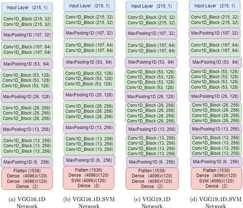
Fig. 13. VGG model architecture.
Figure 13(b) shows that at last block after flatten layer followed by one dense layer SVM is pushed and then output layer has been declared. VGG-16 extracted the features and then SVM finally controlled the optimal hyperplane and eventually gave a better prediction result using 120 neurons. Moreover, Fig. 14 shows the accuracy and loss curves for VGG-16-Conv1D model. In the accuracy graph, the training and validation curves indicate the same behavior. After some epochs, the accuracy curves went to saturation whereas in the loss curve, the validation loss deviates very highly and never went to saturation. This deviation problem has been controlled by applying SVM. Figure 15 illustrates the accuracy and loss after pushing SVM. In contrast, by examining Figs. 14 and 15, it can be said that SVM controls the deviation of the spikes and shows a much better prediction result.
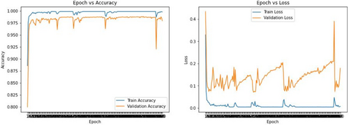
Fig. 14. VGG-16-Conv1D model validation.
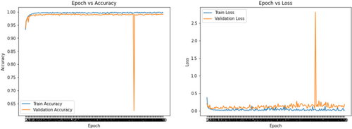
Fig. 15. VGG-16-Conv1D-SVM model validation.
2.3.7. Architecture of VGG-19-Conv1D with SVM
VGG-19, a variant of the VGG model, has a total of 19 layers (16 convolution layers, 3 FC layer, 5 maxpool layers and 1 softmax layer). Like VGG-16, VGG-19 is used to assess the outcome. The architecture of this model in Fig. 13(c) model is briefly described here — a convolutional 1D block has been designed as earlier. Input shape is (215, 1), padding is kept the same throughout the architecture, and kernel initializer used he_normal. The channel was kept to 1 and the filter size was initially set to 32 and gradually increased it exponentially, the feature has been reduced gradually. Also, the FC dense layer in this model used 4096 and 120 neurons, respectively, but 4096 layers didn’t give much satisfactory result so 120 neurons have been used. A total of 19 layers have been used. After the input layer, Conv1D, batch normalization and activation layer have been used. Some maxpooling layers have been used and after flattening the features three dense layers have been used to acquire the classification output. SVM is pushed just before the output dense layer, as shown in Fig. 13(d).
Figure 16 shows that accuracy has remained much different. Validation accuracy has remained low and train accuracy has a significant gap between validation accuracy. On the other hand, the loss curve showed that validation loss was more than training loss and at some point, the deviation from training loss was so high. This deviated behavior has been caused because there is no function to control and thus SVM is integrated later with this model, which is shown in Fig. 17, and it provides better result for prediction.
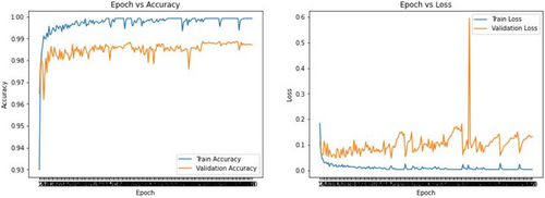
Fig. 16. VGG-19-Conv1D model validation.
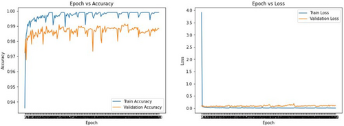
Fig. 17. VGG-19-Conv1D-SVM model validation.
3. Results Analysis and Discussion
This section briefly discusses the obtained result and analysis from the above experiments on acquired dataset.
3.1. Train and test data ratio
Given that the ratio of the training and testing datasets is 80:20, the goal of this experiment was to demonstrate the expected outcome using the learning approach. The training and testing datasets are depicted in Table 1.
| Dataset | Training | Testing | Total Apps |
|---|---|---|---|
| Drebin | 12,024 | 3007 | 15,031 |
3.2. System specifications
One machine with the setup is used to train the models which is shown in Table 2.
| Component | Value |
|---|---|
| CPU | 11th Gen Intel(R) Core (TM) i5-1135G7 @ 2.40GHz |
| GPU | Nvidia RTX 2060 Super GPU |
| RAM | 32GB |
| Disk space | 512GB SSD |
| Metrics | Description |
|---|---|
| TP | Correctly predicts the positive class |
| FP | Incorrectly predicts the positive class |
| TN | Correctly predicts the negative class |
| FN | Incorrectly predicts the negative class |
| Metrics | CNN-1D | DNN | LSTM | RNN | MLP |
|---|---|---|---|---|---|
| Precision | 99.02 | 99.14 | 98.42 | 98.43 | 98.53 |
| Recall | 98.79 | 98.88 | 98.79 | 99.07 | 99.16 |
| F1 score | 98.93 | 99.07 | 98.61 | 98.75 | 98.89 |
| Reference | Modality | Method | Contributions | Performance Metrices and Results |
|---|---|---|---|---|
| Lakshmanarao and Shashi16 | Classification of Android malware | CNN | Android benign and malware APKs are transformed into images and in addition, CNN for DL is suggested | Accuracy: 97.76% with minimal information requirement |
| Singh et al.17 | Deep feature extraction and classification of Android malware images | CNN | Eliminating the feature engineering and domain expert cost | Accuracy: 92.59% using Android certificates and manifest malware images |
| Zhang et al.18 | TCN with bytecode image | TCN | Visual features of the XML file with the data section of the DEX file eases extensive computation | Accuracy: 95.44%, Precision: 95.45%, Recall: 95.45% and F1 score: 95.44% |
| Dina et al.20 | Android malware detection method based on bytecode image | CNN | Encrypted or packed malware can be detected | Accuracy: 95.1% using CNN with high-order feature map |
| Li et al.21 | Android malware detection using DNN | DNN | DeepDetector displays information about each malware family in details and examines its rate of detection | 97% malware detection at 0.1% FP rate and Precision 96% |
| Alzaylaee et al.22 | DL-based Android malware detection through dynamic analysis using stateful input generation | DNN | The findings emphasize the importance of improved input generation for dynamic analysis | 97.8% detection rate (with dynamic features only) and 99.6% detection rate (with dynamic + static features) |
| Jiang et al.23 | Obfuscated Android malware detection | Transfer learning | Identification of obfuscated malware and unobfuscated malware illustration to the obfuscated one | Accuracy 92.26% (obfuscated malware), Accuracy 87.39% for malware family detection and the average detection time spent 0.963s |
| Karbab and Debbabi20 | Adaptive Android malware detection | DL | Addition of family clustering to static analytics using NLP and ML | High detection rate (98–99% F1 score) |
| Proposed model (hybrid approach) | Detection of Android malware | VGG-16-Conv1D-SVM | The hybrid model gives better performance over other models | Precision: 98.56%, Recall: 98.78% and F1 score: 99.20% |
3.3. Performance metrics
Metrics such as Precision, Recall and F1 score are used to evaluate how well DL and hybrid approaches work in identifying malicious Android applications. A well-known method for visualizing the effectiveness of a classification algorithm is the confusion matrix. It consists of four elements: TP — True Positive, FP — False Positive, TN — True Negative and FN — False Negative.
The ratio of the total number of cases properly predicted to the total number of samples is known as accuracy. The ratio of accurately anticipated positive instances to all positively predicted instances is known as precision. While the recall is determined by dividing the total number of positive cases by the proportion of correctly predicted positive instances. The F1 score considers both recall and precision.
3.4. Performance evaluation of the developed models
3.4.1. Evaluating DL models
From earlier research, it has been discovered that some DL techniques are effective for spotting dangerous software while others are not. The MLP, CNN, RNN, DNN and LSTM DL algorithms have all been used in this work. Following model construction, 03 evaluation measures were used to assess performance and choose the most effective classifier for malware detection. Precision for CNN is 99.07%, and recall is 98.79%. Precision in DNN, RNN and MLP is 99.15%, 98.43% and 8.53%, respectively, but it is lower in LSTM at 98.42%. The F1 score creates a single statistic by averaging the harmonics of the precision and recall of a classifier. It is mostly employed to evaluate classifier performance. Assume, for instance, that classifier Y has a greater precision and classifier X has a larger recall. In this situation, it is possible to determine which classifier produces superior results by comparing their F1 scores. By analyzing F1 score, the DNN achieved the highest score with 99.07% and least with LSTM 98.61%. For CNN, RNN and MLP, the F1 scores are 98.93%, 98.75% and 98.89%, respectively. Therefore, DNN, RNN and MLP can be selected for the hybrid model as these are achieved highest scores.
3.4.2. Evaluating hybrid models
The purpose of this research is to illustrate performance evaluation using several hybrid classifiers for detecting Android malware. As previously explained in this study, the SVM algorithm’s goal is to find the optimum decision boundary or line that can categorize the following data points in an n-dimensional space and assign them to that category as rapidly as possible. Classifier performance has increased by using SVM alongside conventional DL models, as demonstrated in Fig. 18. In comparison to conventional models, hybrid LSTM, RNN and MLP models have improved in terms of precision, with the DNN-SVM model having the best accuracy at 99.14%. Additionally, recall is significantly improving. The F1 scores for DNN, RNN and MLP are 99.12%, 98.61% and 99.02%, respectively.
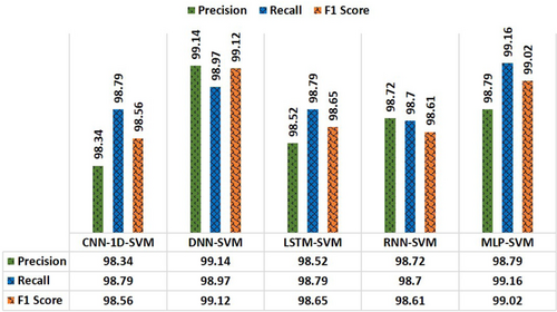
Fig. 18. Results obtained from the hybrid models.
3.4.3. Evaluating VGG models
To assess the classification output in this study, VGG-16 and VGG-19 have also been used. CNN-1D model is uniquely designed for the VGG model. Following flattening and feature extraction for better prediction, SVM is also employed in the dense layer. The VGGNet has three FC layers. Out of the three layers, the first two have 4096 or 120 channels each, i.e., lowering the number of channels in the dense layers, and the third layer outputs 2 channels, 1 for each class, i.e., Malicious or Benign. Using 4096 and 120 channels for FC layers, the classification result was produced which is shown in Figs. 19 and 20. VGG-16-Conv1D-SVM with 120 neurons yields the highest F1 score 99.20% among all VGG models and it was found as the best classifier and architecture of this proposed model is shown in Fig. 21.
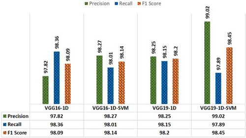
Fig. 19. Performance comparison using 4096 neurons on VGG classifiers.
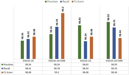
Fig. 20. Performance comparison using 120 neurons on VGG classifiers.
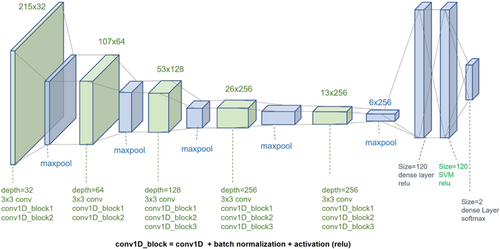
Fig. 21. Proposed model architecture.
Figure 22 depicts the confusion matrices for VGG-16-Conv1D-SVM model and it can be seen there that 1860 samples were accurately identified as benign whereas 1116 samples were identified as malignant for the proposed model. However, a comprehensive overview of similar research outcomes with the proposed model has been further intended to understand the state-of-the-art methodologies and their performance metrics for the classification of Android malware.
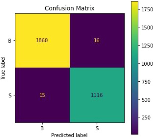
Fig. 22. Confusion matrix for test data for VGG-16-Conv1D-SVM.
4. Conclusion
The goal of this study was to explore several DL algorithms and hybrid approaches for identifying malicious Android applications that utilize static features. Additionally, as our dataset was 1D and was utilized in conjunction with the VGG network to identify malware on Android, we have also put up the novel idea of customizing the VGG model for 1D convolution. Considering the findings of this study in comparison to other works that have been published, this paper offers a new addition to the research community for hybrid approach prediction of harmful Android applications. To the best of our knowledge, the research has shown that the proposed approach is more accurate when compared to other DL and hybrid approaches using reference dataset. This VGG-16 model along with SVM achieves 99.20% F1 score for detecting benign and malicious Android applications.
Future research looks potential for expanding the capabilities of this hybrid technique beyond the two classifications of benign and malicious to include additional labels. Other features in a dynamic way that reflect the activities of malware should also be taken into consideration since we only concentrate on features related to static analysis in this work. Besides, the prediction of Android malware from encrypted and packed Android applications may be the subject of future research. Additionally, a larger dataset can be used to assess the efficacy of the aforementioned method. By first performing a static analysis of the Android applications and then a dynamic analysis, a hybrid solution can be developed which will be an anti-malware that will offer improved security for Android devices.

