Adrenal Tumor Segmentation on U-Net: A Study About Effect of Different Parameters in Deep Learning
Abstract
Adrenal lesions refer to abnormalities or growths that occur in the adrenal glands, which are located on top of each kidney. These lesions can be benign or malignant and can affect the function of the adrenal glands. This paper presents a study on adrenal tumor segmentation using a modified U-Net model with various parameter selection strategies. The study investigates the effect of fine-tuning parameters, including k-fold values and batch sizes, on segmentation performance. Additionally, the study evaluates the effectiveness of different preprocessing techniques, such as Discrete Wavelet Transform (DWT), Contrast Limited Adaptive Histogram Equalization (CLAHE), and Image Fusion, in enhancing segmentation accuracy. The results show that the proposed model outperforms the original U-Net model, achieving the highest scores for Dice, Jaccard, sensitivity, and specificity scores of 0.631, 0.533, 0.579, and 0.998, respectively, on the T1-weighted dataset with DWT applied. These results highlight the importance of parameter selection and preprocessing techniques in improving the accuracy of adrenal tumor segmentation using deep learning.
1. Introduction
Adrenal lesions are growths in the adrenal glands that can be either benign or malignant and are often discovered incidentally during imaging tests. While symptoms may include abdominal pain, high blood pressure, rapid heartbeat, sweating, and anxiety, many adrenal tumors are asymptomatic. The most common type of adrenal tumor is the benign adenoma, which can cause excess hormone production, leading to conditions such as Cushing’s syndrome or primary aldosteronism. Malignant adrenal tumors, such as adrenal cortical carcinoma, are rare but can be aggressive and difficult to treat.1
Segmentation of adrenal lesions from medical images can be a difficult task due to several factors. First, the variability in size and shape of adrenal lesions makes it challenging to develop a single segmentation method that can accurately detect and describe all types of lesions. Second, the varying levels of contrast enhancement in adrenal lesions can impact the accuracy of their detection and segmentation. Additionally, various imaging artifacts, such as motion artifacts, noise, or image distortion caused by patient movement during scanning, can affect the quality of medical images and consequently, the accuracy of adrenal lesion segmentation. Moreover, adrenal lesion segmentation is a subjective process that is dependent on the interpretation and expertise of the radiologist or clinician, which can lead to intra-observer and inter-observer variability. Limited availability of medical image datasets for the development and validation of adrenal lesion segmentation algorithms can also affect their accuracy and generalizability. Lastly, the time-consuming and labor-intensive nature of adrenal lesion segmentation can limit its feasibility in clinical practice. Despite these challenges, the use of advanced machine learning techniques, such as deep learning algorithms, has the potential to improve the accuracy and efficiency of adrenal lesion segmentation.
U-Net is a convolutional neural network architecture that has become popular for its application in medical image segmentation.2 The U-Net architecture comprises a contracting path and a symmetric expanding path, which facilitate contextual and precise localization, respectively. The contracting path is composed of convolutional layers followed by max-pooling operations that gradually reduce spatial resolution while increasing the feature map depth. Conversely, the expanding path comprises up-convolutional layers that increase spatial resolution and reduce feature map depth. The incorporation of skip connections between corresponding layers in the contracting and expanding paths allows the network to concatenate feature maps from different resolutions and retain high-resolution information throughout the segmentation process. U-Net has demonstrated exceptional performance in numerous medical image segmentation tasks due to its ability to capture contextual information and perform precise segmentation.3,4,5,6
In segmentation studies using images where it is difficult to distinguish organs, such as abdominal images, image preprocessing methods and parameter optimization are required to improve the performance of the widely used U-Net model. Image preprocessing is a crucial step that involves the use of techniques to enhance, clean up, or modify digital images before they are analyzed or used for further processing.7 These methods aim to improve the quality of images by removing noise, correcting distortions, and increasing the contrast of images. However, the choice of appropriate parameters is also critical to improving the performance of deep learning models.8 This is because the selection of parameters can significantly affect the accuracy, convergence rate, and generalization ability of the model. Due to the high dimensionality and complexity of deep learning models, the number of parameters involved can be vast, making it challenging to find the optimum configuration. Incorrect selection of parameters can lead to problems such as over or underfitting, which can reduce the performance of the model. Therefore, it is essential to adjust the parameters for specific datasets and tasks to achieve the best results. To select the optimum parameters, a thorough understanding of the model’s architecture, data characteristics, and optimization algorithm used is necessary. The selection of optimum parameters is a crucial step in deep learning model development, which can improve the performance of the model and make it more effective in practical applications.
2. Related Works
Adrenal tumor segmentation studies lack a generally accepted dataset, leading to variations in the datasets used in different studies. Hence, the evaluation of these studies is based on the methodology and performance metrics obtained. Previous adrenal tumor segmentation studies have been performed on abdominal Computer Tomography (CT) and Magnetic Resonance (MR) images. For instance, Tang et al. conducted a segmentation study of heochromocytoma on 10 3D CT images and achieved 92.7% Dice Score Coefficient (DSC) in the arterial phase and 92.9% DSC in the venous phase.9 Chai et al. proposed a computer-aided system consisting of a segmentation algorithm, classification algorithm, and feature extraction for the detection and classification of adrenal tumors on CT images. The study achieved an accuracy of 90% on 436 CT images.10 Koyuncu et al. developed an Adrenal Tumor Segmentation (ATUS) pipeline using a hybrid system of multiple methods for adrenal tumor segmentation in CT images. The study achieved a DSC of 83.06%, Jaccard of 71.44%, sensitivity of 86.44%, specificity of 99.66%, accuracy of 99.43%, and structural similarity index measure (SSIM) of 98.51% using 32 images.11 Zhao et al. utilized a 3D U-Net model to segment adrenal tumor vessels on 49 3D CT images, achieving a DSC of 94.69% and a mean intersection over union (MIoU) of 90.22%.12 Bi et al. used a fully convolutional network (FCN) to detect adrenal tumors on low-contrast CT images and achieved precision, recall, and f-score metrics of 69.82%, 76.29%, and 72.91%, respectively, using 38 low-contrast CT images.13 Barstugan et al. proposed a hybrid method including some image processing methods for the segmentation of adrenal tumors on MR images and achieved a sensitivity, specificity, accuracy, precision, DSC, Jaccard, and SSIM of 60.07%, 99.99%, 97.69%, 83.68%, 63.14%, 51.14%, and 97.07%, respectively, using 113 MR images.14
The current literature on adrenal lesion segmentation is mainly based on CT imaging. However, a recent study is the only known study in the literature to perform adrenal lesion segmentation on MR images.14 Despite both imaging techniques providing detailed images of internal structures, MR offers several advantages over CT for abdominal imaging. MR’s ability to provide superior soft tissue contrast allows for more detailed imaging of abdominal organs and structures, such as the liver, pancreas, and blood vessels, making it particularly useful for detecting and characterizing tumors and other abnormalities, as well as assessing the extent of disease. MR also has the advantage over CT in that it does not use ionizing radiation for abdominal imaging, a significant benefit for patient safety. Abdominal CT studies often require the use of iodine-containing contrast agents, which may be harmful for patients with kidney disease or iodine allergy. In contrast, MR studies typically use safer gadolinium-based contrast agents, which are less harmful for patients with these conditions. Furthermore, MR provides better visualization of certain abdominal structures that may be challenging to image with CT, such as the bile ducts and pancreas. Specifically, MR is the preferred imaging modality for evaluating pancreatic diseases, including tumors and inflammation, due to its ability to provide detailed images of the pancreas and adjacent structures. Finally, MR can provide images in multiple planes, including axial, coronal, and sagittal planes, offering a more comprehensive view of the abdomen. Conversely, CT is mainly limited to providing images in the axial plane, which can complicate the assessment of certain structures within the abdomen.
The literature on this topic reveals several limitations and challenges, including the following:
Data variability: Each dataset used for research is unique, making it difficult to compare studies that use different datasets. Therefore, it is difficult to generalize findings across different datasets.
Limited imaging modalities: Most research in this area has focused on CT imaging. However, the use of CT imaging is limited due to the harmful radiation exposure to patients and the inability to image in multiple planes.
Different thresholds: Studies have employed different thresholds for different types of lesions, which can make it difficult to generalize findings.
Specific target selection: The use of a specific target selection for each image is one of the most significant challenges that limits the generalization of the results to other datasets and populations.
This paper presents a study on the segmentation of adrenal lesions in T1-T2-weighted MR images of the abdomen, using U-Net-based deep learning models as a segmentation approach. In order to enhance the performance of the models, various preprocessing techniques were applied to the images to generate different datasets. Cross-validation was employed during the training phase to avoid potential bias towards a particular subset of the data, which can occur when using a single test set. The most suitable hyperparameter values were determined through cross-validation and batch size selection. The results of this study were compared with state-of-the-art models and different loss functions to reveal the advantages of the proposed method. The significant contributions of the study are as follows:
| (1) | The first study in the literature to perform adrenal lesion segmentation on a previously used dataset, facilitating comparison. | ||||
| (2) | Segmentation of adrenal tumors achieved using deep learning models on T1-T2 weighted abdominal MR images. | ||||
| (3) | Improved segmentation performance and determination of the appropriate image enhancement technique for abdominal images by applying different image enhancement techniques. | ||||
| (4) | The proposed model achieved better results than the original model after modifying the U-Net layers. | ||||
| (5) | Hyperparameters were tuned to obtain optimal values instead of fixed values by varying cross-validation and batch size values. | ||||
| (6) | robustness was demonstrated when compared with state-of-the-art models and models using different loss functions. | ||||
3. Materials and Methods
3.1. Dataset
In this study, a dataset of T1-T2 weighted abdominal MR images of 107 patients acquired with a 2013 model SIEMENS AREA 1.5 T MR unit at the Faculty of Medicine, Department of Radiology, Selcuk University was used. The use of relevant data was discussed at the Non-Interventional Clinical Research Ethics Committee Meeting, Faculty of Medicine, Selcuk University dated 26 July 2017; Approval was obtained with the decision of the board numbered 2017/216 on the subject. The original images were in DICOM format and were converted to JPEG format with a resolution of 800×584 pixels, 8-bit depth, and a DPI of 96. Adrenal lesions in the MR images were identified by expert radiologists from the Department of Radiology, Faculty of Medicine, Selcuk University and were represented as white on the ground truth images while the background was black. Regions of interest (ROIs) were extracted from the images to improve the accuracy and efficiency of data analysis and to reduce the computational load. Figure 1 illustrates the extracted ROI regions from T1-T2 weighted images and examples of ground truth masks corresponding to adrenal lesions in these images.
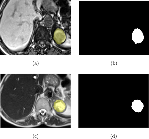
Fig. 1. Images used in the study (a) T1-weighted ROI image, (b) Ground truth mask of T1-weighted ROI image, (c) T2-weighted ROI image, and (d) Ground truth mask of T2-weighted ROI image.
3.2. Image enhancement
In medical imaging, image enhancement techniques play a crucial role in improving the quality and clarity of images to aid in accurate diagnosis and treatment planning. Medical images are often susceptible to various factors, including noise, distortion, and artifacts, which can obscure significant details and make it difficult to identify pathological features. By reducing these effects and improving contrast, sharpness, and overall image quality, image enhancement techniques can improve the visual interpretability of medical images.
This study applies different image enhancement methods, such as Discrete Wavelet Transform (DWT), Contrast Limited Adaptive Histogram Equalization (CLAHE), and Image Fusion (Max Fusion and Average Fusion), to the datasets used and compares the effectiveness of each method.
3.2.1. Discrete wavelet transform
Discrete wavelet transform (DWT) is widely used in medical imaging to enhance image quality, by improving contrast, sharpness, and overall image appearance. DWT-based image enhancement techniques have the potential to reduce image noise, remove artifacts, and enhance fine details, thus facilitating more accurate diagnostic interpretation.15
DWT is a mathematical technique that decomposes an image into different frequency components called wavelets. Figure 2 provides an example of a 2-level DWT, where an input signal (X[n]) is subjected to a low pass filter (LPF), which produces an approximation component (A), while a high pass filter (HPF) produces a detail component (D). This decomposition process is then repeated, generating further frequency resolution approximation components, which are once again down-sampled by passing through the LPF and HPF, ultimately resulting in 2-level DWT components. Figure 3 shows examples obtained by applying this process to the images used in this study.
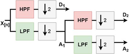
Fig. 2. 2-Level discrete wavelet transform.
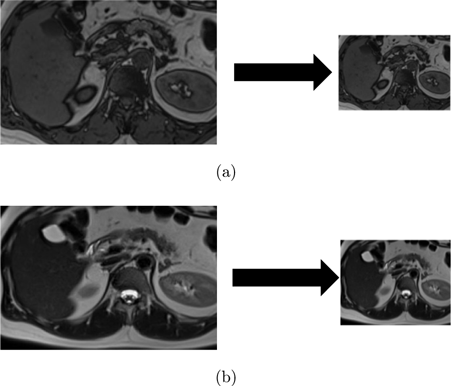
Fig. 3. (a) T1-weighted image and corresponding image after 2-level DWT, and (b) T2-weighted image and corresponding image after 2-level DWT.
3.2.2. Contrast limited adaptive histogram equalization
Contrast limited adaptive histogram equalization (CLAHE) is a common technique for medical image enhancement. This method improves the contrast of an image by redistributing the pixel values of the image through a histogram equalization algorithm.15 Unlike traditional histogram equalization, CLAHE adjusts the contrast enhancement locally to different regions of the image. This adaptive technique enables it to process images more effectively with varying contrast levels, such as medical images with uneven lighting or contrast. To achieve this, the image is divided into small regions, and the histogram of each region is calculated and equalized individually.16 The block diagram illustrating the CLAHE process steps is presented in Fig. 4, and examples of T1-T2 weighted abdominal images obtained by applying CLAHE to the dataset used in the study are shown in Fig. 5.
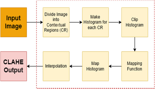
Fig. 4. CLAHE overall block diagram.
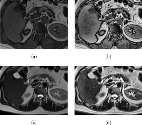
Fig. 5. (a) T1-weighted image, (b) CLAHE result of T1-weighted image, (c) T2-weighted image, and (d) CLAHE result of T2-weighted image.
3.2.3. Image fusion
In medical imaging, image fusion is a technique used to integrate multiple images of the same scene acquired from different sensors or modalities into a single composite image that contains more comprehensive information than the individual images. The goal of image fusion is to improve the visual quality of the images, increase useful information, and facilitate better diagnosis or treatment planning.7
Various methods are available for image fusion in medical imaging, including maximum fusion, mean fusion, and principal component analysis (PCA). The maximum fusion approach is a straightforward method that selects the maximum intensity value from each corresponding pixel in the input images. On the other hand, the mean fusion method calculates the mean intensity value. PCA is a more complex approach that employs a mathematical transformation to maximize the variance of the resulting image.
In this study, a wavelet transform-based fusion approach is utilized. The fusion process is executed using the MATLAB wavelet analyzer toolbox, and both maximum fusion and mean fusion techniques are implemented, specifying the type of wavelet used being specified. After performing a 2-level db2 wavelet transform on the input images, fusion datasets are generated via both techniques. Figure 6 illustrates the series of steps involved in the image fusion process and shows the resulting images obtained through this process.
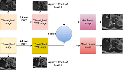
Fig. 6. Max and mean fusion images from T1-T2 weighted images.
3.3. Segmentation models
3.3.1. U-Net
The U-Net model is a widely used neural network architecture for medical image segmentation. The model employs an encoder-decoder structure with skip connections between the encoder and the corresponding decoder layers to address the challenge of preserving spatial information during image segmentation.2
The encoder consists of multiple convolutional blocks, each consisting of two 3×3 convolutional layers, followed by a rectified linear unit (ReLU) activation function and a 2×2 max pooling layer. The number of filters in each block doubles after each max pooling layer to increase the receptive field of the network and capture more complex features.
The decoder has the same number of blocks as the encoder, but each block is replaced by an up-sampling layer followed by concatenation with the corresponding feature map from the encoder. The concatenated feature maps are then passed through two 3×3 convolutional layers with ReLU activation. Finally, a 1×1 convolution is applied to map the feature vector to the required number of classes.
The U-Net model uses binary cross-entropy loss, which is commonly used for binary segmentation tasks. The number of filters in the first convolutional layer is typically set to 64 and doubles after each pooling layer. However, this can be adjusted according to the size and complexity of the input images.
Figure 7 depicts the block diagram of the original U-Net model, illustrating the encoder, decoder, and skip connections between them.
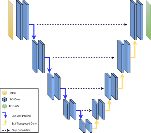
Fig. 7. U-Net block diagram.
3.3.2. Modified U-Net
The proposed modified U-Net model differs from the original U-Net model in two main aspects. First, the Parametric Rectified Linear Unit (PReLU) is used as the activation function in the layers instead of the ReLU used in the original model. PReLU allows the activation function to learn the negative slope of the function, unlike ReLU, which has a fixed slope of zero. This feature enables PReLU to adapt to the input data and leads to better performance in tasks such as image classification and object detection. Additionally, PReLU addresses the problem of “dying ReLU” by preventing the gradients in the network from going to zero for certain inputs, thus improving the learning capacity of the network.
Second, the Dice loss function is used instead of the binary cross-entropy loss function used in the original model. Dice loss is based on the Dice similarity coefficient, a statistical measure that quantifies the similarity of two datasets. The Dice similarity coefficient is defined as twice the intersection of two sets divided by the sum of their sizes. Dice loss has various advantages over binary cross-entropy loss in medical image segmentation tasks. First, it is better suited for unbalanced datasets because it penalizes false negatives and false positives equally, resulting in better performance on unstable datasets. Second, it provides a smoother optimization environment and is less likely to get stuck at the local minimum, leading to better results. Finally, Dice loss encourages better segmentation by penalizing false negatives and false positives equally, leading to more accurate segmentation results and better preservation of small structures.
The proposed U-Net has a similar architecture to the model shown in Fig. 7. Nevertheless, it distinguishes itself from the original model in terms of the activation and loss functions employed. The efficacy of these modifications will be evaluated through the results obtained from the study.
3.4. Evaluation metrics
In the field of machine learning, evaluation metrics play a crucial role in objectively measuring the performance of models or algorithms in solving specific problems. These metrics help to evaluate the accuracy, efficiency, and robustness of the model or algorithm. In the context of medical image segmentation, various evaluation metrics are used to assess different aspects of the study. For example, Dice Similarity Coefficient (DSC), Jaccard Index (JI), Sensitivity (Sens), and Specificity (Spec) are some of the commonly used metrics to evaluate medical image segmentation studies. These metrics are defined using parameters such as True Positive (TP), True Negative (TN), False Positive (FP), and False Negative (FN), as expressed in Eqs. (1)–(4)17:
In the later stages of the study, an additional evaluation metric, Hausdorff Distance (HD), was included to compare the performance of the proposed model with the state-of-the-art models and different loss functions. HD is a metric that measures the maximum distance between any point on the predicted mask and the closest point on the ground truth mask. It is particularly useful for evaluating the segmentation accuracy of complex structures. The mathematical formulation of HD is presented in Eq. (5), and a visual representation of the HD metric is provided in Fig. 8.18
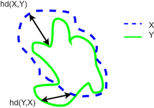
Fig. 8. (Color online) Components of the calculation of the Hausdorff Distance between the green line X and the blue line Y.19
3.5. Loss functions
Loss functions are essential in medical image segmentation to measure the difference between the predicted segmentation mask and the ground truth mask. The appropriate selection of the loss function can significantly impact the accuracy and convergence rate of the segmentation model. Several commonly used loss functions in medical image segmentation include binary cross-entropy loss, dice loss, focal loss, Tversky loss, and Tversky focal loss. Binary cross-entropy (BCE) loss is effective for binary partitioning tasks, while dice loss is suitable for unstable datasets with unbalanced foreground and background pixels. Focal loss emphasizes hard-to-classify samples to solve the issue of class imbalance. Tversky loss, a variant of dice loss, includes two additional hyperparameters to control the weight given to false positives and false negatives.20 Finally, Focal Tversky loss integrates the concepts of both Focal and Tversky loss to reduce the contribution of easy pixels and place more emphasis on misclassified hard pixels.21 The choice of loss function depends on the particular medical image segmentation task at hand. The mathematical expressions of the loss functions are given in Eqs. (6)–(10):
The proposed model in this study employs the Dice loss function. Subsequently, models with alternative loss functions were trained using the best-performing parameters, and the results were subsequently compared.
4. Experiments
The experiments were conducted on a computer system equipped with an Intel€ X€ (R) E-2236 CPU running at a clock speed of 3.40GHz, 32GB of RAM, and an NVIDIA GeForce GTX 1660 TI graphics card. All experiments were performed on the Windows 10 operating system using TensorFlow 1.14 framework version, with the Adam optimizer. The learning rate was reduced by 10% when there was no improvement every 3 epochs, with the learning rate varying from 10−3 to 10−5. The study was conducted according to the following flow:
The images in the dataset were pre-processed and different datasets were created, including raw and pre-processed datasets.
The dataset was divided into three sets, namely, training, validation, and test sets, based on the cross-validation values determined for the training processes. Data augmentation was applied to the training data to prevent overfitting. Specifically, 10% of the data allocated to the training set was reserved for validation.
The training was carried out using both the original U-Net model and the proposed model. The training was repeated for different batch sizes to determine the optimal batch size.
After training, the trained models were tested on the test images, and their performance was evaluated using the chosen evaluation metrics.
Figure 9 shows example images of the data augmentation while Fig. 10 shows the workflow of the study. The values of the parameters used to train the models are shown in Table 1.
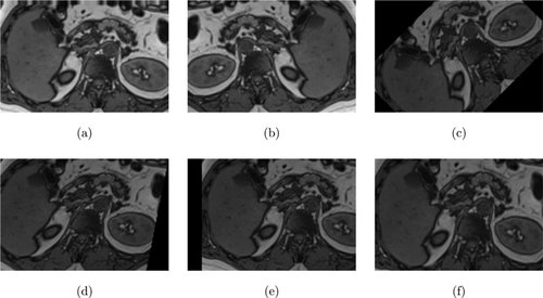
Fig. 9. (a) Height shift, (b) Horizontal flip, (c) Rotation, (d Shear, (e) Width shift, and (f) Zoom.
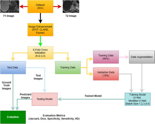
Fig. 10. Flowchart of the study.
| Loss Functions | BCE Loss, Dice Loss |
| Learning Rate | 1e−4:1e−5 |
| Optimizer | Adam |
| Activation Function | ReLU, PReLU |
| Epochs | 1000 |
| Cross-validation | 2, 3, 4 |
| Batch Size | 1, 2, 3, 4, 5 |
5. Results
This section presents the quantitative results obtained from training the original U-Net and the proposed model, which are categorized under different subheadings based on the type of dataset used, including, T1–T2 weighted datasets with preprocessed datasets, and fusion datasets. The performance metrics evaluated include DSC, JI, sensitivity (Sens), and specificity (Spec), using the original (RAW), DWT, and CLAHE applied datasets with three different cross-validation values (k=2, 3, 4) and five different batch sizes (1, 2, 3, 4, 5). Finally, an overall evaluation of all studies is presented, and the findings are discussed.
5.1. Quantitative results of T1-weighted images
This study evaluated the performance of the original U-Net model trained on T1-weighted abdominal images and preprocessed datasets, using varying batch sizes and k-fold values, and the average test results are presented in Table 2. The findings revealed that when the RAW dataset was employed, the performance decreased with increasing batch size across all k-fold values for each metric. Notably, the best results for all metrics were observed when k=3 was selected for the RAW dataset.
| RAW | DWT | CLAHE | ||||||||
|---|---|---|---|---|---|---|---|---|---|---|
| Batch | Metrics | k=2 | k=3 | k=4 | k=2 | k=3 | k=4 | k=2 | k=3 | k=4 |
| 1 | DSC | 0.456 | 0.583 | 0.504 | 0.517 | 0.600 | 0.524 | 0.398 | 0.500 | 0.431 |
| JI | 0.362 | 0.476 | 0.403 | 0.419 | 0.516 | 0.432 | 0.311 | 0.397 | 0.335 | |
| Sens | 0.379 | 0.545 | 0.415 | 0.461 | 0.516 | 0.385 | 0.306 | 0.470 | 0.300 | |
| Spec | 0.379 | 0.998 | 0.997 | 0.997 | 0.997 | 0.997 | 0.998 | 0.998 | 0.998 | |
| 2 | DSC | 0.422 | 0.514 | 0.497 | 0.451 | 0.608 | 0.543 | 0.391 | 0.482 | 0.441 |
| JI | 0.329 | 0.412 | 0.399 | 0.361 | 0.509 | 0.448 | 0.306 | 0.388 | 0.346 | |
| Sens | 0.300 | 0.487 | 0.381 | 0.397 | 0.529 | 0.420 | 0.280 | 0.440 | 0.309 | |
| Spec | 0.998 | 0.998 | 0.998 | 0.996 | 0.997 | 0.996 | 0.998 | 0.997 | 0.998 | |
| 3 | DSC | 0.393 | 0.537 | 0.472 | 0.442 | 0.611 | 0.472 | 0.354 | 0.520 | 0.446 |
| JI | 0.302 | 0.446 | 0.380 | 0.355 | 0.507 | 0.383 | 0.268 | 0.414 | 0.343 | |
| Sens | 0.288 | 0.502 | 0.332 | 0.460 | 0.531 | 0.336 | 0.278 | 0.468 | 0.311 | |
| Spec | 0.990 | 0.998 | 0.998 | 0.991 | 0.998 | 0.998 | 0.981 | 0.998 | 0.997 | |
| 4 | DSC | 0.397 | 0.513 | 0.470 | 0.475 | 0.566 | 0.508 | 0.352 | 0.469 | 0.428 |
| JI | 0.309 | 0.421 | 0.372 | 0.373 | 0.472 | 0.416 | 0.267 | 0.376 | 0.331 | |
| Sens | 0.318 | 0.478 | 0.352 | 0.567 | 0.504 | 0.367 | 0.319 | 0.443 | 0.308 | |
| Spec | 0.965 | 0.997 | 0.994 | 0.963 | 0.998 | 0.998 | 0.978 | 0.998 | 0.992 | |
| 5 | DSC | 0.383 | 0.474 | 0.425 | 0.455 | 0.565 | 0.481 | 0.358 | 0.432 | 0.428 |
| JI | 0.289 | 0.378 | 0.333 | 0.364 | 0.464 | 0.387 | 0.268 | 0.331 | 0.330 | |
| Sens | 0.281 | 0.438 | 0.341 | 0.508 | 0.518 | 0.445 | 0.306 | 0.483 | 0.382 | |
| Spec | 0.997 | 0.998 | 0.949 | 0.983 | 0.994 | 0.996 | 0.971 | 0.974 | 0.961 | |
Interestingly, for the models trained on the DWT applied data, the best results were obtained with different batch sizes for each k-fold value. Specifically, the optimal results for all metrics were obtained with the combination of k=3 and batch 3 combination. Moreover, the models trained on the CLAHE applied data demonstrated an increase in performance as the k value increased. Additionally, it was observed that the optimal results for this dataset were obtained with the same combination as DWT.
Overall, the results suggest that among the different preprocessed datasets, the DWT applied dataset demonstrated superior performance in terms of all the evaluation metrics considered.
Table 3 presents the average test results obtained from the training of the proposed U-Net model on T1-weighted abdominal datasets. The results indicate that a decrease in metrics is observed when a high batch size (4 and 5) is selected for all k-fold values.
| RAW | DWT | CLAHE | ||||||||
|---|---|---|---|---|---|---|---|---|---|---|
| Batch | Metrics | k=2 | k=3 | k=4 | k=2 | k=3 | k=4 | k=2 | k=3 | k=4 |
| 1 | DSC | 0.471 | 0.554 | 0.491 | 0.485 | 0.631 | 0.523 | 0.426 | 0.497 | 0.463 |
| JI | 0.373 | 0.454 | 0.398 | 0.393 | 0.533 | 0.430 | 0.332 | 0.393 | 0.364 | |
| Sens | 0.349 | 0.530 | 0.364 | 0.474 | 0.579 | 0.375 | 0.312 | 0.465 | 0.327 | |
| Spec | 0.998 | 0.998 | 0.995 | 0.996 | 0.998 | 0.998 | 0.998 | 0.997 | 0.998 | |
| 2 | DSC | 0.455 | 0.573 | 0.491 | 0.461 | 0.631 | 0.524 | 0.416 | 0.513 | 0.531 |
| JI | 0.356 | 0.466 | 0.395 | 0.375 | 0.525 | 0.433 | 0.321 | 0.409 | 0.434 | |
| Sens | 0.353 | 0.538 | 0.331 | 0.453 | 0.574 | 0.364 | 0.327 | 0.455 | 0.366 | |
| Spec | 0.997 | 0.998 | 0.998 | 0.996 | 0.997 | 0.998 | 0.998 | 0.998 | 0.997 | |
| 3 | DSC | 0.429 | 0.533 | 0.468 | 0.482 | 0.612 | 0.537 | 0.394 | 0.495 | 0.438 |
| JI | 0.337 | 0.439 | 0.376 | 0.382 | 0.508 | 0.437 | 0.302 | 0.398 | 0.340 | |
| Sens | 0.339 | 0.512 | 0.335 | 0.486 | 0.552 | 0.357 | 0.282 | 0.458 | 0.336 | |
| Spec | 0.998 | 0.998 | 0.998 | 0.992 | 0.998 | 0.998 | 0.997 | 0.998 | 0.996 | |
| 4 | DSC | 0.408 | 0.476 | 0.463 | 0.452 | 0.599 | 0.502 | 0.371 | 0.507 | 0.443 |
| JI | 0.317 | 0.385 | 0.369 | 0.364 | 0.492 | 0.411 | 0.282 | 0.408 | 0.347 | |
| Sens | 0.433 | 0.451 | 0.317 | 0.435 | 0.536 | 0.417 | 0.326 | 0.461 | 0.306 | |
| Spec | 0.988 | 0.997 | 0.996 | 0.995 | 0.997 | 0.997 | 0.947 | 0.998 | 0.998 | |
| 5 | DSC | 0.369 | 0.488 | 0.443 | 0.449 | 0.597 | 0.503 | 0.344 | 0.470 | 0.414 |
| JI | 0.281 | 0.393 | 0.351 | 0.356 | 0.492 | 0.408 | 0.259 | 0.368 | 0.321 | |
| Sens | 0.482 | 0.465 | 0.332 | 0.469 | 0.536 | 0.354 | 0.386 | 0.475 | 0.348 | |
| Spec | 0.913 | 0.993 | 0.968 | 0.982 | 0.995 | 0.998 | 0.941 | 0.966 | 0.959 | |
Notably, the results suggest that the best results are obtained when 3-fold cross-validation is used in datasets other than the CLAHE applied dataset. Specifically, the combination of 3-fold cross-validation and batch 1 yielded the optimal performance for the DWT applied dataset, as presented in Table 3. Moreover, in terms of performance, the DWT applied dataset demonstrated the best performance, followed by the RAW and CLAHE datasets, respectively.
This part aimed to evaluate the impact of various preprocessing techniques on the performance of segmentation models trained on T1-weighted images. The findings indicate that the DWT applied dataset yielded the best results, followed by the RAW and CLAHE applied datasets, respectively. Thus, it can be inferred that DWT application has a positive effect on T1-weighted images, while CLAHE application has a negative effect.
Interestingly, the optimal performance for both models was achieved when using 3-fold cross-validation, although with different batch sizes. Furthermore, the proposed segmentation model outperformed the original model. Specifically, when 3-fold cross-validation and batch 1 were selected with the proposed model trained on the DWT dataset, the DSC, JI, sensitivity, and specificity metrics yielded values of 0.631, 0.533, 0.579, and 0.998, respectively, representing the best results.
5.2. Quantitative results of T2-weighted images
In this section, the results of the model training conducted on T2-weighted abdominal images are presented. Initially, the original U-Net model was trained on the datasets, and the results are shown in Table 4. The results show that the best results were obtained when batch 1 was selected for all k values in the RAW dataset. Three-fold cross-validation was observed to be the most effective technique.
| RAW | DWT | CLAHE | ||||||||
|---|---|---|---|---|---|---|---|---|---|---|
| Batch | Metrics | k=2 | k=3 | k=4 | k=2 | k=3 | k=4 | k=2 | k=3 | k=4 |
| 1 | DSC | 0.412 | 0.482 | 0.470 | 0.318 | 0.417 | 0.391 | 0.425 | 0.398 | 0.475 |
| JI | 0.320 | 0.392 | 0.375 | 0.245 | 0.332 | 0.310 | 0.331 | 0.306 | 0.373 | |
| Sens | 0.321 | 0.383 | 0.307 | 0.188 | 0.280 | 0.276 | 0.349 | 0.248 | 0.276 | |
| Spec | 0.997 | 0.999 | 0.999 | 0.999 | 0.999 | 0.999 | 0.999 | 0.999 | 0.998 | |
| 2 | DSC | 0.378 | 0.450 | 0.454 | 0.326 | 0.393 | 0.354 | 0.362 | 0.436 | 0.468 |
| JI | 0.292 | 0.359 | 0.359 | 0.252 | 0.302 | 0.280 | 0.280 | 0.342 | 0.374 | |
| Sens | 0.344 | 0.356 | 0.238 | 0.195 | 0.291 | 0.212 | 0.330 | 0.273 | 0.265 | |
| Spec | 0.997 | 0.999 | 0.998 | 0.999 | 0.998 | 0.999 | 0.999 | 0.999 | 0.999 | |
| 3 | DSC | 0.300 | 0.443 | 0.440 | 0.284 | 0.384 | 0.367 | 0.329 | 0.340 | 0.427 |
| JI | 0.230 | 0.355 | 0.347 | 0.217 | 0.296 | 0.293 | 0.258 | 0.262 | 0.338 | |
| Sens | 0.413 | 0.433 | 0.378 | 0.218 | 0.267 | 0.232 | 0.286 | 0.214 | 0.213 | |
| Spec | 0.872 | 0.998 | 0.995 | 0.996 | 0.999 | 0.999 | 0.995 | 0.999 | 0.999 | |
| 4 | DSC | 0.374 | 0.435 | 0.400 | 0.314 | 0.377 | 0.371 | 0.337 | 0.431 | 0.415 |
| JI | 0.284 | 0.343 | 0.317 | 0.236 | 0.296 | 0.291 | 0.260 | 0.334 | 0.328 | |
| Sens | 0.353 | 0.388 | 0.282 | 0.167 | 0.254 | 0.264 | 0.181 | 0.274 | 0.293 | |
| Spec | 0.998 | 0.998 | 0.998 | 0.998 | 0.999 | 0.998 | 0.999 | 0.999 | 0.998 | |
| 5 | DSC | 0.300 | 0.373 | 0.389 | 0.257 | 0.334 | 0.341 | 0.305 | 0.328 | 0.409 |
| JI | 0.224 | 0.291 | 0.310 | 0.187 | 0.252 | 0.262 | 0.232 | 0.250 | 0.320 | |
| Sens | 0.338 | 0.534 | 0.331 | 0.275 | 0.235 | 0.332 | 0.259 | 0.294 | 0.246 | |
| Spec | 0.978 | 0.895 | 0.998 | 0.961 | 0.998 | 0.986 | 0.979 | 0.981 | 0.999 | |
In the case of the DWT applied dataset, batch 2 for k=2, and batch 1 for the others demonstrated the best performance. On the other hand, for the CLAHE applied dataset with batch 2 for 3-fold cross-validation and batch 1 for the remaining k values provided the optimal results.
In summary, the results in Table 4 suggest that the optimal performance, as indicated by all the metrics, was achieved by using 3-fold cross-validation and batch 1 with RAW dataset.
Table 5 shows the performance results attained by training with the proposed model. The highest performance scores were observed when batch 1 was chosen for all cross-validation values in both the RAW and DWT applied datasets. For the CLAHE dataset, batch 4 exhibited the best results for 3-fold cross-validation, while batch 1 yielded optimal performance for other cross-validation values. Especially, the optimal performance across all evaluated datasets was achieved with 3-fold cross-validation and batch 1 in the RAW dataset.
| RAW | DWT | CLAHE | ||||||||
|---|---|---|---|---|---|---|---|---|---|---|
| Batch | Metrics | k=2 | k=3 | k=4 | k=2 | k=3 | k=4 | k=2 | k=3 | k=4 |
| 1 | DSC | 0.430 | 0.503 | 0.470 | 0.376 | 0.434 | 0.399 | 0.399 | 0.395 | 0.486 |
| JI | 0.333 | 0.405 | 0.375 | 0.291 | 0.339 | 0.317 | 0.311 | 0.308 | 0.391 | |
| Sens | 0.360 | 0.366 | 0.280 | 0.291 | 0.293 | 0.268 | 0.276 | 0.243 | 0.257 | |
| Spec | 0.997 | 0.998 | 0.998 | 0.998 | 0.999 | 0.999 | 0.999 | 0.999 | 0.999 | |
| 2 | DSC | 0.412 | 0.476 | 0.462 | 0.338 | 0.378 | 0.370 | 0.376 | 0.407 | 0.433 |
| JI | 0.319 | 0.378 | 0.370 | 0.263 | 0.300 | 0.297 | 0.290 | 0.315 | 0.342 | |
| Sens | 0.343 | 0.405 | 0.344 | 0.236 | 0.264 | 0.220 | 0.285 | 0.258 | 0.258 | |
| Spec | 0.998 | 0.999 | 0.998 | 0.998 | 0.999 | 0.999 | 0.998 | 0.999 | 0.998 | |
| 3 | DSC | 0.364 | 0.447 | 0.417 | 0.355 | 0.376 | 0.372 | 0.343 | 0.397 | 0.449 |
| JI | 0.281 | 0.356 | 0.332 | 0.276 | 0.290 | 0.296 | 0.265 | 0.312 | 0.353 | |
| Sens | 0.384 | 0.372 | 0.328 | 0.193 | 0.248 | 0.233 | 0.260 | 0.227 | 0.284 | |
| Spec | 0.993 | 0.999 | 0.998 | 0.998 | 0.998 | 0.999 | 0.999 | 0.999 | 0.999 | |
| 4 | DSC | 0.383 | 0.447 | 0.430 | 0.305 | 0.371 | 0.382 | 0.371 | 0.427 | 0.405 |
| JI | 0.297 | 0.351 | 0.345 | 0.229 | 0.290 | 0.300 | 0.282 | 0.326 | 0.325 | |
| Sens | 0.356 | 0.365 | 0.357 | 0.170 | 0.252 | 0.273 | 0.326 | 0.276 | 0.217 | |
| Spec | 0.999 | 0.999 | 0.998 | 0.999 | 0.999 | 0.998 | 0.947 | 0.999 | 0.999 | |
| 5 | DSC | 0.293 | 0.394 | 0.436 | 0.307 | 0.371 | 0.365 | 0.329 | 0.363 | 0.426 |
| JI | 0.218 | 0.301 | 0.349 | 0.233 | 0.288 | 0.288 | 0.253 | 0.278 | 0.331 | |
| Sens | 0.488 | 0.333 | 0.372 | 0.174 | 0.262 | 0.232 | 0.193 | 0.234 | 0.247 | |
| Spec | 0.857 | 0.980 | 0.998 | 0.992 | 0.999 | 0.999 | 0.999 | 0.998 | 0.998 | |
The aim of this section was to compare the performance of two segmentation models on T2-weighted images with different datasets, including RAW, CLAHE, and DWT applied datasets. The obtained results demonstrated that the RAW dataset outperformed the other preprocessed datasets for both models, followed by the CLAHE and DWT applied datasets, respectively. These results indicate that the preprocessing techniques did not have a positive effect on the T2-weighted images.
Furthermore, the optimal combination for both models was 3-fold cross-validation and batch 1. It is noteworthy that the proposed segmentation model exhibited superior performance compared to the original model. Specifically, when using the RAW dataset was used with the proposed model, the best results were achieved with DSC of 0.503, JI of 0.405, sensitivity of 0.366, and specificity of 0.998.
To summarize, the results of this investigation suggest that the RAW dataset with the proposed segmentation model and the combination of 3-fold cross-validation and batch 1 could provide the most favorable results for segmenting adrenal lesions on T2-weighted images.
5.3. Quantitative results of fusion images
This section presents the results of the segmentation models trained on the datasets obtained from the fusion processes conducted on T1 and T2-weighted MR images. The study employed both maximum and mean fusion techniques, and the outcomes are reported in Table 6 for both models.
| U-Net | Modified U-Net | ||||||||||||
|---|---|---|---|---|---|---|---|---|---|---|---|---|---|
| Max fusion | Mean fusion | Max fusion | Mean fusion | ||||||||||
| Batch | Evaluation metrics | k=2 | k=3 | k=4 | k=2 | k=3 | k=4 | k=2 | k=3 | k=4 | k=2 | k=3 | k=4 |
| 1 | DSC | 0.373 | 0.473 | 0.429 | 0.317 | 0.484 | 0.447 | 0.362 | 0.426 | 0.444 | 0.294 | 0.348 | 0.404 |
| JI | 0.290 | 0.384 | 0.340 | 0.238 | 0.391 | 0.356 | 0.268 | 0.337 | 0.341 | 0.209 | 0.261 | 0.305 | |
| Sens | 0.265 | 0.373 | 0.239 | 0.285 | 0.435 | 0.323 | 0.276 | 0.363 | 0.251 | 0.234 | 0.206 | 0.354 | |
| Spec | 0.998 | 0.999 | 0.998 | 0.996 | 0.999 | 0.997 | 0.997 | 0.999 | 0.998 | 0.996 | 0.999 | 0.997 | |
| 2 | DSC | 0.337 | 0.479 | 0.448 | 0.317 | 0.469 | 0.364 | 0.342 | 0.367 | 0.410 | 0.285 | 0.443 | 0.406 |
| JI | 0.265 | 0.371 | 0.355 | 0.240 | 0.378 | 0.287 | 0.256 | 0.272 | 0.314 | 0.206 | 0.339 | 0.312 | |
| Sens | 0.247 | 0.404 | 0.239 | 0.296 | 0.402 | 0.312 | 0.264 | 0.285 | 0.234 | 0.306 | 0.345 | 0.329 | |
| Spec | 0.997 | 0.998 | 0.998 | 0.995 | 0.999 | 0.997 | 0.997 | 0.998 | 0.999 | 0.997 | 0.999 | 0.997 | |
| 3 | DSC | 0.306 | 0.426 | 0.390 | 0.310 | 0.417 | 0.414 | 0.229 | 0.403 | 0.390 | 0.277 | 0.422 | 0.390 |
| JI | 0.234 | 0.345 | 0.311 | 0.230 | 0.330 | 0.323 | 0.163 | 0.317 | 0.299 | 0.199 | 0.325 | 0.298 | |
| Sens | 0.373 | 0.344 | 0.221 | 0.346 | 0.314 | 0.335 | 0.201 | 0.351 | 0.224 | 0.347 | 0.338 | 0.329 | |
| Spec | 0.953 | 0.999 | 0.998 | 0.956 | 0.999 | 0.997 | 0.961 | 0.999 | 0.997 | 0.981 | 0.999 | 0.998 | |
| 4 | DSC | 0.285 | 0.430 | 0.424 | 0.297 | 0.450 | 0.368 | 0.264 | 0.392 | 0.380 | 0.274 | 0.427 | 0.373 |
| JI | 0.212 | 0.348 | 0.335 | 0.228 | 0.357 | 0.290 | 0.198 | 0.307 | 0.292 | 0.200 | 0.335 | 0.279 | |
| Sens | 0.177 | 0.344 | 0.218 | 0.333 | 0.371 | 0.326 | 0.198 | 0.319 | 0.210 | 0.326 | 0.379 | 0.300 | |
| Spec | 0.995 | 0.998 | 0.998 | 0.995 | 0.999 | 0.997 | 0.997 | 0.999 | 0.999 | 0.996 | 0.999 | 0.998 | |
| 5 | DSC | 0.269 | 0.374 | 0.375 | 0.268 | 0.414 | 0.379 | 0.292 | 0.324 | 0.363 | 0.281 | 0.402 | 0.344 |
| JI | 0.200 | 0.294 | 0.293 | 0.199 | 0.321 | 0.293 | 0.208 | 0.247 | 0.282 | 0.199 | 0.308 | 0.256 | |
| Sens | 0.234 | 0.384 | 0.292 | 0.397 | 0.411 | 0.343 | 0.307 | 0.255 | 0.231 | 0.352 | 0.454 | 0.333 | |
| Spec | 0.992 | 0.973 | 0.965 | 0.953 | 0.994 | 0.995 | 0.961 | 0.995 | 0.978 | 0.986 | 0.986 | 0.998 | |
Upon evaluating the study results on a model basis, it was observed that batch 1 provided the best results for 2-fold cross-validation in the original model for the maximum fusion dataset, while batch 2 yielded optimal performance for the other datasets. Conversely, for the mean fusion dataset, batch 2 yielded the best results for 2-fold cross-validation, while batch 1 was found to be optimal for the other datasets.
Additionally, the results indicate that the best performance was achieved when k=3 was selected for both datasets in this model. Specifically, the DSC, JI, sensitivity, and specificity metrics yielded the best results for the mean fusion applied dataset with a DSC value of 0.484, JI value of 0.391, sensitivity value of 0.435, and specificity value of 0.999, when 3-fold cross-validation and batch 1 were utilized.
Based on the results obtained with the proposed model, it is observed that batch 1 is the most effective choice for all cross-validation values in the maximum fusion dataset, and batch 1 is the optimal choice for the mean fusion dataset with 2-fold cross-validation, whereas batch 2 is preferred for the others. Regarding the datasets, the best performance is achieved when 4-fold cross-validation is applied to the maximum fusion dataset and 3-fold cross-validation is used for the mean fusion dataset. The most successful results are obtained with 4-fold cross-validation and batch 1, according to the trainings performed with the recommended model. The performance metrics are recorded as DSC, JI, sensitivity, and specificity 0.444, 0.341, 0.251, and 0.998, respectively.
When comparing the training performed on the fusion datasets with both models, it was noted that the original model outperformed the recommended model. However, the performance of the original model was found to be inferior to that of other preprocessing techniques, namely DWT and CLAHE.
5.4. Evaluation of quantitative results
The study aimed to investigate the effects of different models, preprocessing techniques, k-fold values, and batch sizes on adrenal lesion segmentation performance. The results showed that the original U-Net model outperformed the proposed model in fusion datasets, while the proposed model performed better in other datasets. Among the datasets used, the DWT-applied T1-weighted images, RAW T2-weighted images, and average fusion images showed better results. The best performance was achieved when 3-fold cross-validation and batch 1 were selected for all datasets, which is a critical criterion for parameter determination.
Table 7 presents the best results obtained for each dataset, including the addition of the Hausdorff Distance (HD) metric. Remarkably, the pair of cross-validation and batch size that yielded the best results was common to all datasets. When comparing performance across datasets, the T1-weighted dataset outperformed the T2-weighted and mean fusion images, respectively. Furthermore, it was observed that the proposed model outperformed the original model by a significant margin. The best results were achieved on the T1-weighted dataset with DWT applied, with DSC, JI, sensitivity, specificity, and HD metrics yielding values of 0.631, 0.533, 0.579, 0.998, and 2.95mm, respectively, when 3-fold cross-validation and batch 1 were selected in the proposed model.
| Metrics | |||||||
|---|---|---|---|---|---|---|---|
| Dataset | Parameters | Model | DSC | JI | Sens | Spec | HD (mm) |
| T1-(DWT) | k:3-B:1* | Modified (PReLU) U-Net | 0.631 | 0.533 | 0.579 | 0.998 | 2.950 |
| T2-(RAW) | k:3-B:1* | Modified (PReLU) U-Net | 0.503 | 0.405 | 0.366 | 0.998 | 2.854 |
| Mean Fusion | k:3-B:1* | U-Net | 0.484 | 0.391 | 0.435 | 0.999 | 2.716 |
6. Discussion
This section aims to demonstrate the robustness of the proposed model by comparing it with state-of-the-art models and different loss functions in U-Net. For this purpose, all models were trained on the DWT dataset, which yielded the most successful results in this study, while 3-fold cross-validation and batch 1 were selected. State-of-the-art models including DeepLabV3 Plus,22 SegNet,23 and U-Net++5 were chosen for comparison. Furthermore, BCE, Tversky, and Focal-Tversky loss functions were used as alternative loss functions for the proposed model.
In Table 8,24 the results of the conducted training using state-of-the-art models and different loss functions are presented. The proposed methods with distinct loss functions, such as BCE loss in model A, Tversky loss in model B, and Focal-Tversky loss in model C, are demonstrated. In addition, the study by Barstugan et al.,14 which also conducted segmentation on the same dataset as this study, is included for comparison purposes. The table provides evaluation metrics along with the number of parameters and training times for the models.
| Metrics | |||||||
|---|---|---|---|---|---|---|---|
| Model | DSC | JI | Sens | Spec | HD (mm) | Training parameters (millions) | Training time |
| DEEPLAB V322 | 0.557 | 0.457 | 0.477 | 0.997 | 2.427 | 17.83 | 15:16:21 |
| SEGNET23 | 0.576 | 0.459 | 0.522 | 0.995 | 2.013 | 2.941 | 3:13:06 |
| U-NET++5 | 0.566 | 0.474 | 0.518 | 0.997 | 3.060 | 8.193 | 13:58:29 |
| Barstugan et al.14 | 0.631 | 0.511 | 0.600 | 0.998 | — | — | — |
| Proposed Model* | 0.631 | 0.533 | 0.579 | 0.998 | 2.950 | 36.535 | 12:45:01 |
| Model A* | 0.416 | 0.327 | 0.320 | 0.995 | 3.167 | 36.535 | 12:25:05 |
| Model B* | 0.500 | 0.402 | 0.382 | 0.995 | 3.030 | 36.535 | 12:16:35 |
| Model C* | 0.499 | 0.404 | 0.383 | 0.995 | 3.166 | 36.535 | 12:17:01 |
After analysis of the findings in Table 8 based on the metrics used, the following conclusions can be drawn. In terms of the DSC metric, the highest performance is achieved by Barstugan et al. and the proposed model, followed by SegNet and U-Net++. Models B and C have moderate DSC scores, while Model A has the lowest DSC scores. For the JI metric, the proposed model has the highest score, followed by Barstugan et al., and Model A has the lowest JI score. The sensitivity and specificity measures indicate the superior ability of the proposed model to detect the presence or absence of objects in the image. The HD measures the maximum distance between the points of the two sets, with lower HD scores indicating better performance. According to the HD metric, SegNet has the best performance, followed by the proposed model, while Models A, B, and C have relatively high HD scores. The proposed model has the highest number of parameters, while SegNet has the lowest number of parameters, indicating its ability to achieve comparable performance with fewer parameters. Finally, the time metric shows the time required to train each model, with the proposed model having the highest training time, followed by Model A, and SegNet having the lowest training time.
The comparison of quantitative results demonstrates the superiority of the proposed model over state-of-the-art models, different loss functions, and related studies. This alone confirms the robustness of the proposed model. To further develop the analysis and improve the reliability of the comparison, a qualitative comparison is also included in this section. For this purpose, the image outputs of the trained models and the proposed model on the test images are presented, and the DSC of each predicted image is calculated for comparison to remove subjectivity and ensure objective evaluation. The qualitative comparison results, presented in Table 9, show that the proposed model outperforms all other models both visually and mathematically for all images.
The findings obtained as a result of the conducted studies have been compared both with existing studies in the literature and with different state-of-the-art models. Tables 8 and 9 provide quantitative and qualitative evaluations, respectively. In both tables, it is evident that the proposed model outperforms other methods.
| Predictions | ||||||||
|---|---|---|---|---|---|---|---|---|
| Test image | Ground truth | Modified U-Net (Dice Loss) | Modified U-Net (BCE Loss) | Modified U-Net (Tversky Loss) | Modified U-Net (Focal-Tversky Loss) | DeepLab V3 | U-Net ++ | SegNet |
 |  |  DSC=0.945 DSC=0.945 |  DSC=0.822 DSC=0.822 |  DSC=0.940 DSC=0.940 |  DSC=0.835 DSC=0.835 |  DSC=0.831 DSC=0.831 |  DSC=0.776 DSC=0.776 |  DSC=0.854 DSC=0.854 |
 |  |  DSC=0.974 DSC=0.974 |  DSC=0.956 DSC=0.956 |  DSC=0.958 DSC=0.958 |  DSC=0.950 DSC=0.950 |  DSC=0.851 DSC=0.851 |  DSC=0.973 DSC=0.973 |  DSC=0.868 DSC=0.868 |
 |  |  DSC=0.937 DSC=0.937 |  DSC=0.895 DSC=0.895 |  DSC=0.876 DSC=0.876 |  DSC=0.909 DSC=0.909 |  DSC=0.903 DSC=0.903 |  DSC=0.833 DSC=0.833 |  DSC=0.716 DSC=0.716 |
 |  |  DSC=0.809 DSC=0.809 |  DSC=0.704 DSC=0.704 |  DSC=0.723 DSC=0.723 |  DSC=0.776 DSC=0.776 |  DSC=0.699 DSC=0.699 |  DSC=0.533 DSC=0.533 |  DSC=0.657 DSC=0.657 |
7. Conclusion
The aim of this study was to adrenal lesion segmentation on T1-T2-weighted MR images of the abdomen by proposing a new model and testing different preprocessing techniques, k-fold cross-validation, and batch sizes to identify the optimal framework for achieving the best performance.
The preprocessing techniques employed included DWT, CLAHE, and max-mean fusion processes. The study found that DWT preprocessing on T1-weighted images outperformed the raw dataset for T2-weighted images, and the fusion datasets had the least successful results. Among all datasets, the T1-weighted dataset with DWT applied yielded the best results. In terms of k-fold cross-validation, 3-fold cross-validation gave the best results, followed by 4-fold and 2-fold cross-validation, respectively. The study observed a significant decrease in work performance at high batch numbers (4,5), and the best results were generally obtained with batch 1. The proposed model gave by far the best performance, as shown by both quantitative and qualitative comparisons with various state-of-the-art models and loss functions.
The study also revealed hardware-based limitations that prevented trying higher values for k-fold cross-validation and batch size. Future studies are planned to improve the proposed model and perform different analyses.
ORCID
Ahmet Solak  https://orcid.org/0000-0002-5494-1987
Rahime Ceylan  https://orcid.org/0000-0003-0294-5692
Mustafa Alper Bozkurt  https://orcid.org/0000-0001-5171-3295
Hakan Cebeci  https://orcid.org/0000-0002-2017-3166
Mustafa Koplay  https://orcid.org/0000-0001-7513-4968

