Hyperparameter Optimization of a Parallelized LSTM for Time Series Prediction
Abstract
Long Short-Term Memory (LSTM) Neural Network has great potential to predict sequential data. Time series prediction is one of the most popular experimental subjects of LSTM. To this end, various LSTM algorithms have been developed to predict time series data. However, there are a few works considering the hyperparameter optimization of LSTM along with parallelization approaches. To address this problem, a parallelized classic LSTM is proposed to predict time series. In the preprocessing phase, it first replaces missing values with zero and then normalizes the time series matrix. The transposed matrix is divided into training and testing parts. Consequently, a core-based parallelism is established, thereby utilizing forking to split prediction into multiple processes. Derivative-free optimization techniques are also analyzed to find out what sort of hyperparameter optimization technique is much more feasible for a parallelized LSTM. Further, a state-of-the-art comparison is included in the study. Experimental results show that training loss is optimal when using Nelder–Mead. Employing effort-intensive optimization methods such as genetic algorithms results in a remarkable CPU time reduction in parallelized designs according to the results. Last, the proposed algorithm outperformed the comparison methods with respect to the prediction errors.
1. Introduction
1.1. Motivation
Time series data analysis has grown at a fast pace in the last decade thanks to the rapid advance in data collection techniques.1,2,3 The techniques predicting time series were first developed for univariate data. But they require strong preprocessing4,5,6,7 in this field. Feature selection is a typical problem when working with data sets having a lot of features. Auto-Regressive Integrated Moving Average model (ARIMA) and its derivatives dominate univariate time series prediction researche.8,9,10 However, ARIMA is computationally expensive if there is a need for feature selection. Further, such models are focused on backward data rather than turning points of time series. In addition to this, ARIMA has configurable parameters that determine the way it works. These parameters should be configured during the pre-training phase to build a reliable prediction model. However, in some cases, the results might not be biased in favor of hyperparameter optimization as in LSTM.
LSTM has played an increasingly significant role in predicting sequential data.11,12,13,14 Related studies are mainly focused either on modifying its structure to increase prediction performance or comparing LSTM with its alternatives. LSTM further provides a multivariate time series prediction.15,16,17 It has the following advantages over the alternatives:
| (1) | LSTM can handle noisy data, | ||||
| (2) | It can work with an unlimited number of states contrary to the finite state models, | ||||
| (3) | LSTM is highly flexible to adapt fine-tuning so that it enables us to search hyperparameters in a large space. | ||||
A parallelized classic LSTM (PCLSTM) is developed in this study. PCLSTM consists of three major processes: preprocessing, establishing core-based parallelism, and prediction. In the preprocessing, missing values are eliminated and then a min-max normalization is conducted. Subsequently, core-based parallelism is established by utilizing R parallel package. The parallelization encompasses hyperparameter optimization and time series prediction in producing the ultimate results. Instead of performing an experiment having a narrow scope, this work analyzes the effects of hyperparameter optimization on PCLSTM by using derivative-free optimization methods. To this end, a maximization-based Bayesian optimization method is further devised. What makes our study distinctive from the preceding works is that our experiment includes a comprehensive derivative-free analysis in finding optimal settings of an LSTM.
1.2. Contribution
This study claims the contributions presented as follows:
| (1) | To reduce the prediction time, a new parallelized LSTM is devised. | ||||
| (2) | The question this paper tries to answer is: “What type of derivative-free optimization methods is effective in reducing central processing unit (CPU) time in parallel architecture?” | ||||
| (3) | To our knowledge, this study is the first to investigate to what extent can derivative-free optimization methods helps reduce the errors of LSTM in predicting time series. | ||||
| (4) | The proposed method includes a maximization-based Bayesian optimization approach for regression. | ||||
2. Background
2.1. Time series prediction
Given a data space R, X is the feature set of R in which it can be labeled with Y. However, in time series prediction, each feature should be associated with a time point t=1,…,Tt=1,…,T. f(σt):Xt→Ytf(σt):Xt→Yt is the mapping function to expose the training data to a learning process. The distribution of the labels reflects the model of YtYt values. In f(σt)f(σt), each previous prediction for t−1t−1 point bolsters the prediction conducted at t. In that process, we aim to keep the error of prediction f(Rt)=EYt∼Xt[L(f(Xt,σ),Yt]f(Rt)=EYt∼Xt[L(f(Xt,σ),Yt] to a minimum in which L denotes the loss produced from σσ of parameter space. To minimize the risk of time series analysis, we adopt Invariant Causal Prediction (ICP).18
2.2. Core-based parallelism
There are four types of parallelization: data-based,19 model-based,20 spatial,21 and reduction-based parallelism.22 Since it provides data-based parallelism, in this paper, we choose core-based parallelism to divide the data into multiple cores. Since we do not use online data, communication cannot be considered as a performance bottleneck to sustain reliable synchronization.
Given a set of cores C1,…,CnC1,…,Cn in which n is the number of cores to be used to establish explicit parallelism. An input X is divided into n parts sequentially. For instance, the first part is assigned to core 1, n−1n−1th part to n−1n−1th core.
2.3. Hyperparameter optimization
Let ω1,…,ωtω1,…,ωt a set of machine learning algorithms where Υ1,…,ΥzΥ1,…,Υz are the available tuning methods that are suitable to apply those algorithms. Each ΥΥ may produce a distinctive tuning time ΔΔ depending on the structural properties of ΥΥ. The optimal tuning time can be represented with Υ∗Υ∗ that is chosen from a large result space. Each cost of ΥΥ is computed with ∑zi=1△i∗Pi∑zi=1△i∗Pi in which P is coefficient to yield the related cost. The main purpose of the tuning process is to enhance the efficiency of general effect max(∏zi=1Pi△i)max(∏zi=1Pi△i).
2.4. Recurrent neural networks
RNN is a special type of feed-forward neural network that has internal memory to keep input. For that reason, this subsection intends to detail RNN from which LSTM is derived.
RNN provides a powerful alternative for predicting the patterns of sequential data.23 Text sequence prediction24,25,26 and speech recognition27,28,29 are the main application areas of RNN. It gives each output as input to the hidden layers which generates a memorizing mechanism. RNN is much more useful in time series prediction because each hidden layer remembers its previous input. If a classification is performed with RNN, it assumes that features are somehow correlated. For that reason, training RNN takes far more time than other types of deep learning. If the previous state and input state are represented with psps and isis, respectively. The current state cscs of an RNN can be formulated with the following function :
Figure 1 shows the basic structure of an LSTM unit in which FtFt denotes the forget gate at a specific time t. Input gate ItIt and output gate OtOt are also in the same frame. Here σσ represents the activation function in which processed input nodes XtXt are analyzed. Cell state c and the hidden layer h are given together in the structure. Using those terms, the following calculations are performed :
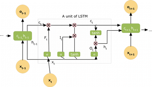
Fig. 1. Overview of a classic LSTM.
2.5. Derivative-free optimization
This subsection describes four derivative-free optimization methods that differ in various details that shape the experiment with an adaptive parallelization. Derivative-free optimization methods generally require a lot of function evaluations so an adaptive parallelization30 is adopted in this study.
Random search prefers to find parameters in various distinct places depending on the number of parameters.31 If the time allocated for hyperparameter optimization is limited, random search could be a possible way to reduce optimization time. Further, parallelization can be easily established in a random search as it does not require communication between workers. The following equation describes the computational complexity of random search :
Genetic algorithm. Three concepts constitute the mechanism of evolution: natural selection,32 mutation,33 and genetic.34 Combining these three concepts resulted in the genetic algorithm which is useful for any optimization problem. The main objective of the genetic algorithm is to find a global optimum by searching a space including many local optimums. For that reason, it requires a large number of computations. The genetic algorithm utilizes mutation that leads to varying outcomes in which the problem is not adaptable to differentiable or continuous objective functions. The complexity of the genetic algorithm is given in Eq. (11) in which P denotes the population size, g is the number of generations, and m represents the size of individuals
Bayesian optimization. Bayes’ theorem is directly related to Bayesian optimization. It builds a probabilistic model by assuming a past event which is a base to evaluate a current event. The approximation of Bayes is called a surrogate function that is used for future sampling. In Bayesian optimization, the acquisition criterion decides which sample will be selected in the next evaluation.35 The complexity of Bayesian optimization is
Nelder–Mead optimization, which is very effective for stochastic responses, was first introduced in 1965.36 Nelder–Mead performs an iterative computation to complete optimization at a low cost. It aims at minimizing the error e of an objective function f(x). Here x is a member of the solution space and f(x) is updated for each response as follows :
Nelder–Mead has rarely been examined along with hyperparameter optimization. It evaluates the optimization results depending on the size of the search space. That issue has been removed by utilizing parallel computation methods. On the other hand, Bayes is much more compatible with parallelization. In each iteration, attaining the desired accuracy at one or two function evaluations can be considered a major advantage of Nelder–Mead.
3. Related Work
ARIMA may be a possible solution when developing a univariate model. It is mainly employed in predicting time series that have one feature associated with the time. Conducting the prediction through one variable requires a feature selection process. Therefore, the works utilizing ARIMA generally present some sophisticated methods associated with feature selection.
Domingos et al.37 developed an ARIMA method that performs a linear and nonlinear calculation, thereby utilizing the neural network more effectively. The method addresses those calculations as a two-step approach that outperformed various methods such as support vector regression. Missing value imputation is one of the important problems of time series prediction. To address this issue, Cao et al.38 proposed a data-covering technique that was able to reduce error propagation by conducting a two-way checking system.
LSTM can be considered an effective method in predicting time series since it holds the information of current and previous inputs. Sagheer and Kotb14 proposed a deep-architecture LSM for predicting the production data of petroleum. The method yielded a relatively low root mean square error (RMSE) compared to the models such as ARIMA that employ univariate time series. Evolutionary computation is a supportive method that helps increase the performance of LSTM. Li et al.39 presented an evolutionary computation technique based on the random search to find optimal hyperparameters of LSTM. The method produced higher accuracy than those of its competitors in moving data sets. LSTM has been rarely implemented in relational data. In such a study,40 a method based on LSTM was developed to predict relational time series. The method has two distinctive properties: (1) It establishes a Spatio-Temporal cell between two LSTM models, and (2) It has a fusion module that gathers information about the last Spatio-Temporal cell. Error rates of the method are even lower than those of ARIMA and convolutional LSTM. Financial data was tried in LSTM due to their compatibility in constructing time series. For instance, Li and Li41 proposed a novel LSTM that is highly sensitive to the noise of the time series. Their method achieved higher regression scores than those of support vector machine (SVM) and multi-layer perceptron (MLP).
Although it is widely assumed that hyperparameter optimization has crucial for machine learning algorithms, very few studies analyzed the effects of hyperparameter optimization on LSTM. Greff et al.42 investigated nine different LSTM methods on three data sets in terms of hyperparameter tuning. According to that study, the learning rate is the most important hyperparameter and the size of the hidden layers follows it. Moreover, the study found that vanilla LSTM is superior to the other types of LSTM in terms of classification error.
Reimers and Gurevych43 observed the efficacy of tuning hyperparameters of LSTM in ordered labeling. According to the obtained results, the chosen optimizer and the classifier used as the last layer should be regarded to increase the performance. On the other hand, the number of the recursive unit was found to be less effective compared to the other types of hyperparameters. The time passed to complete optimization is an inevitable disadvantage of methods producing high accuracy. Differential evolution is a good example of such a method. Therefore, Nakisa et al.44 stressed that the burden originating from hyperparameter optimization can be alleviated via either the cloud or parallel computation.
Breuel45 built an experiment realizing a specific analysis that is related to a peephole connection in the performance of LSTM. He detected that classic LSTM has various advantages over other types of LSTM in classification. He also depicted that some hyperparameters including peephole, momentum, and batch size have not a remarkable effect in tuning the performance of LSTM. Evolutionary computation is eligible for optimizing hyperparameters of LSTM. A genetic algorithm was thus utilized to configure five hyperparameters of LSTM in a study conducted by Gorgolis et al.46
Karim et al.11 tried to increase the performance of LSTM in classification with the help of a convolutional structure. They utilized the Adam optimizer to find a suitable configuration of hyperparameters. Although they achieved clear success in the reduction of classification error, the computational burden in terms of CPU time was disregarded in their experiment. Bandara et al.47 devised a new decomposition technique for LSTM to predict seasonal models of time series. Although their method yielded promising results in terms of mean absolute scaled error (MASE), the method was not improved with high-performance computing. A real-time Kalman filter model (OSAF+AKF) was presented in Ref. 48. The main purpose of that study is to predict seasonal heteroscedasticity in time series. However, the study did not consider any tuning process for the hyperparameters of OSAF+AKF. Chen et al.49 developed a parallel time series prediction algorithm namely periodicity-based parallel time series prediction (PPTSP) for periodic data patterns. The parallelization of PPTSP was implemented in Apache Spark because it holds data in RAM without requiring a distribution operation. That algorithm was able to produce a lower root mean square error (RMSE) than those of the five comparison methods. As the number of computation nodes increases, the decline of the average execution time of PPTSP slows down. Further, tuning times of the hyperparameter of PPSTP were not evaluated on a cloud computing system. Tan et al.50 proposed an adaptive prediction method (TDAP) for time series. In a classification experiment, a high area under the curve (AUC) was yielded, thereby parallelizing TDAP on Apache Spark. However, hyperparameter tuning was disregarded in the construction of TDAP.
In Ref. 51, a parallel cooperation search algorithm (PCSA) is developed for time series forecasting. PCSA is a divide-and-conquer technique in that small-sized groups of the population are shared among multiple threads. The best solution is achieved by the main thread determined at the beginning of the algorithm. Nevertheless, PCSA cannot guarantee the optimal model due to the local convergence problem. Guo et al.52 combined convolutional neural networks (CNNs) with LSTM to predict train travel times. The method was devised based on a parallel deep learning scheme that takes advantage of bidirectional input data. In the comparison performed with six baseline techniques, the method yielded the smallest prediction error. But the study did consider the configurable hyperparameters of neither CNN nor LSTM. In Ref. 53, a parallel neuro-fuzzy algorithm was proposed to predict multivariate time series data. Although the method was able to produce promising results even for recurrent data models, the genetic algorithm employed to configure the initialization phase of the experiment was not evaluated with other types of tuning methods. Parallel models were integrated with a sophisticated hybridization method for time series forecasting in Ref. 54. The proposed method conducted modeling by merging complementary hybrid schemes. In that way, the main limitation of traditional approaches was bypassed, thereby involving the remaining patterns that were ignored in the modeling. However, that study did not consider various hyperparameter configurations of competitive techniques. Li et al.55 developed a parallel reservoir algorithm for multivariate data. The study stressed that involving the correlation between variables results in high prediction accuracy. However, their method cannot respond to fast changes in states. A hybrid technique56 including four linear and nonlinear models is proposed for wind power forecasting. The method leverages a special Kalman filter that does not eliminate critical data while removing residuals. Although the proposed method outperformed two competitive techniques in MAE and RMSE, the study did not consider tuning ARIMAX before establishing parallelization with multilayer perceptron. A parallel design of reservoirs significantly accelerates time-series prediction with the help of quantum computing.57 But to achieve generalizable results, the cross-gain coefficient should be tuned according to the type of delay to yield a minimum error. Table 1 gives concise information on the most associated studies including time series analysis. Note that there are relatively few works leveraging hyperparameter optimization to increase the success of time series forecasting.
| Ref. | Year | Research objective | HO |
|---|---|---|---|
| 51 | 2022 | To develop a parallel forecasting system for time series | No |
| 52 | 2022 | To design a parallel network model for travel time prediction | No |
| 53 | 2022 | To propose a parallel fuzzy network for multi-step time series | Yes |
| 54 | 2022 | To integrate parallel models with hybridization for time series forecasting | No |
| 55 | 2022 | To design multi-parallel cycle reservoirs for time series | No |
| 56 | 2022 | To devise a hybrid method for wind power forecasting | No |
| 57 | 2022 | To propose a parallel design of reservoir for time series prediction | No |
| 49 | 2019 | To develop a periodicity-based parallel algorithm for time-series | No |
| 46 | 2019 | To propose an evolutionary HO technique for recurrent models | Yes |
| 58 | 2021 | To perform prediction of non-stationary time series data a parallel mechanism is proposed | No |
4. Method
4.1. Parallelization
The architecture employed for parallelizing LSTM is presented in Fig. 2. According to that design, time series data is split into small files in the first step. The number of these files is equal to the number of cores. In that process, small parts are constituted by the instances rather than features. The number of cores is detected to pursue parallelization. In the third step, the number of input blocks is determined depending on the number of cores. Fork() function, which is only run on Linux systems, is called to create sub-processes. Each core divides the related input into some threads to perform time series prediction. All the results are then collected from those cores to evaluate the general result.
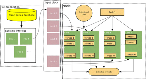
Fig. 2. Parallelization architecture employed for LSTM.
To realize parallelization, mclapply, which is a function of the parallel package in R, is utilized to establish computation. It is easy to use and reduces overhead, remarkably. mclapply is only run on one machine having a great number of cores instead of utilizing various machines as some other parallelization functions do. That is the main drawback of mclapply.
4.2. PCLSTM
Let n be the features of m the observations in a matrix M, the size of the matrix is n×m for multivariate time series prediction. The label count is thus limited to m. Preprocessing is crucial to apply a prediction process to time series data. For this reason, an imputation is performed with zero if the related value is not available (NA). The missing value rate (MVR) is then calculated as follows :
To normalize the values of a time series matrix, the formula utilized to apply range normalization is
Training is executed for 200 iterations. Each data set is divided into three parts: train, validation, and test. After defining the elements of the LSTM unit, arrays are exploited by inference function taking three parameters including data, symbol, and model argument. The iteration is executed depending on the length of prediction that is set to the sequential length of the LSTM.
The iteration performed in a specific timestamp can be formulated as follows :
Let Ψ be the prediction length. The number of samples Δ is used to create arrays on the training data which is taken from the data set. trainData and trainLabel constitute two parts of the training data. The inference function is represented with μ and ϕ predicts the inferred data. ϑ is utilized to generate training arrays in which R and T are temporary variables to add new values that came from the inference function.
Actual and predicted values are evaluated by using Eq. (16) which results in two lists obtained via previous states of LSTM. The general outline of the PCLSTM is given in Algorithm 1 that utilizes Eqs. (15) and (16) to complete prediction. PCLSTM is parallelized by obeying the architecture given in Fig. 2. M←mclapply(M) implies that the data set is divided into the cores which the experimental machine has. For this reason, Steps 5–29 of PCLSTM are repeated for each one of the cores. In Step 5, the null values are assigned to zero. The range normalization is conducted between Steps 6–14 for each cell of the time series matrix that is transposed in Step 15. The matrix is then divided into arrays in compliance with the batch size of LSTM in Step 16. The training data is chosen and exposed to training, validation, and testing processes in Steps 17–30. Last, the prediction result is returned in Step 32.

4.3. Maximization-based Bayesian optimization
This study proposes a maximization-based Bayesian optimization technique given in Algorithm 2 that takes four parameters as input. The algorithm runs depending on the bayesIteration and H. For each iteration, two lists (result1,result2) are generated by using actual and predicted values. Sums of these values are then calculated. scoreList is constituted by conducting a mod operation with those sums. Last, the maximum result is found in score to return optimal H.

5. Experiment
The codes devised to conduct the experiment are publicly availablea for replication purposes. In order to create symbols of LSTM, mxnet library59 of R was utilized. That library also employs an internal optimization during the iterations of training. The settings of the internal optimizer are set as follows: optimizer=AdaDelta,60 decay rate=0.9, optimizer constant:1e−06, regularization coefficient:1e−06, rescaling factor:1/batch size. Unlike other types of optimizers such as Adagrad, AdaDelta does not decrease the learning rate sharply thanks to the evaluation of past 10 gradients instead of involving all the gradients for specific time steps. This is the reason why we employ AdaDelta for internal optimization. To initialize the iterator of array input, mx.init.Xavier function is used. The distribution of the weights is set to Gaussian since the time series matrix is exposed to the normalization process in the previous step of Algorithm 1.
5.1. Dataset
In the experiment, two groups of time series data were processed and predicted with the comparison methods including PCLSTM. The first group includes weather status values of Brazilian cities (Natal, Sao Paulo, Porto Alegre, and Manaus). Each data set consists of 312 samples and six features. The features recorded for each month from January 1990 to December 2015 are as follows: cloudiness, rainfall, max temperature, min temperature, humidity, and mean temperature. The aim here is to predict the mean temperature of each month. The data set is available at https://github.com/ASOCD-ataSets/Weather-DataSet for the general use of practitioners.
Sudeste, which is hourly weather data gathered from the southern region of Brazil, constitutes the second group. It has 31 features and 9.800.000 instances. The data set can be obtained via https://www.kaggle.com/rtatma-n/reading-in-sudeste-csv-file. The mean temperature of Sudeste is subjected to the prediction. Since the size of Sudeste is very large (1.72 GB) for time series prediction, 50.000 instances are taken for each prediction. To that end, the results of 196 data parts are combined to reach a general bias.
5.2. Baselines
ARIMA has been involved in the comparison methods due to its simple yet effective solution61 for univariate data. Since it copes with one feature, each data set is converted to the form as follows: Index, time, and value. The mean temperature is chosen depending on each month of the records. Three terms including p, d, and q are tuned with the derivative-free optimization. They decide the number of autoregressive terms, the degree to which used nonseasonal difference, and the number of lagged forecasting errors, respectively. The range of those employed in the tuning process is as follows: 1–3, 1–3, and 1–3 for step size (1).
Holt–Winters is a well-known alternative for univariate data. The Holt–Winters method62 performs an exponential smoothing on time series data. It can also handle the changes in trends and seasonal parts of the time series. The Holt–Winters is very useful to detect the general behavior of the time series being analyzed. The behavior may be an error trend, seasonal effects, or specific trends. Weighting coefficients chosen for the optimization are as follows: α, β, and γ. α is the filtering parameter. β determines the level of exponential smoothing. Whether the model is seasonal or not is decided with γ. The range used for these hyperparameters is 0.1–0.9 for the step size (0.1).
Online seasonal adjustment factors plus adaptive Kalman filter (OSAF+AKF)48 was devised for predicting seasonal patterns of time series. To that end, the Kalman filter was utilized to detect volatility in time series. We added OSAF+AKF to the comparison methods because it showed great promise within online models. The range used for determining p, d, and q is as follows: (1–3, Step size:1).
Periodicity-based Parallel Time Series Prediction (PPTSP)49 was developed for predicting periodicity in time series. PPTSP tends to show high scalability with time series data. It yielded relatively low RMSE as well. The most intriguing aspect of the study is that it includes a comprehensive parallelization for time series on Apache Spark. Four hyperparameters employed for morphological similarity measurement were analyzed as follows: growth step (μ): 5–40, Step size: 1, inflection points (φ): 0.1–0.9, step size: 0.1.
5.3. Experimental settings
The experiment has a two-fold validation. First, a machine having a 2.4GHz Xenon (X3430) CPU, 8GB Ram, and Windows 10 operating system is employed to predict time series without utilizing parallelization. Second, a parallel design is established on a mainframe having 32 CPU(s), Intel(R) Xeon(R) CPU E5-2690, 222 GB Ram, CentOS 7 operating system, and NVIDIA Tesla S870 graphic card.
Each data set is divided into three parts: training, validation, and testing. 70%, 15%, and 15% are the rates of division, respectively. First, training is completed on 70% of a data set. The validation part is then used to configure hyperparameters. Last, the overall result is achieved in the testing part. These processes are repeated 200 times to obtain an average result.
To evaluate the training and losses of the derivative-free optimization methods, mean square error (MSE) is recorded depending on the number of epochs :
Table 2 gives the details of tuned hyperparameters. It is clear that the genetic algorithm prefers a high dropout rate compared to the other methods. Contrary to that method, Bayesian optimization was completed with low dropout rates. The number of stacked and hidden layers is similar to the comparison methods.
| Method | Manaus | Natal | PortoAlegre | SaoPaulo | Sudeste |
|---|---|---|---|---|---|
| Bayesian optimization | 3–0.11–9 | 4–0.12–14 | 3–0.19–15 | 3–0.15–17 | 5–0.1–16 |
| Genetic algorithm | 4–0.55–11 | 4–0.31–15 | 3–0.42–13 | 3–0.89–15 | 4–0.53–12 |
| Nelder–Mead | 5–0.24–10 | 3–0.60–14 | 2–0.60–11 | 4–0.1–15 | 5–0.3–15 |
| Random search | 4–0.34–11 | 3–0.8–15 | 2–0.47–13 | 5–0.4–12 | 4–0.13–16 |
For Bayesian optimization, we chose the settings: initial points=2, steps of Bayesian optimization=1, and kappa=2.576. In the genetic algorithm, the settings chosen are as follows: type = real-valued, population size=50, number of generations=10, elitism=2, crossover probability=0.8, mutation probability=0.1. The stopping criterion of Nelder–Mead is set to 1e−06 and the maximum number of evaluations is 1000. However, the number of iterations of Nelder–Mead changes between 50–60 depending on the scale of the data set.
6. Results
The values given in Table 3 were obtained by averaging the results of all the experimental data sets. It is worth noting that multivariate prediction of time series resulted in low errors compared to those of univariate prediction. Concretely, ARIMA and Holt–Winters have yielded at least 1.1 higher RMSE than the other methods. The case is not different for the other measures but the difference is very between ARIMA and the multivariate methods. However, Holt–Winters yielded relatively better results than ARIMA. PCLSTM was found to be the best for performance measures among the comparison methods. On the other hand, PPTSP produced the second-lowest prediction errors. OSAF+AKF is preferable when the results are evaluated with MAE and MPE. To reduce the error, multivariate prediction is a solution in which the structure of data sets is compatible with that type of analysis.
| Method | RMSE | MAE | MPE | MAPE |
|---|---|---|---|---|
| ARIMA | 10.28633 | 52.85161 | 37.30992 | 40.72708 |
| Holt–Winters | 8.21632 | 34.11223 | 22.45313 | 29.22099 |
| OSAF+AKF | 7.10345 | 5.56786 | 2.74501 | 15.34567 |
| PPTSP | 5.14561 | 6.45891 | 3.23412 | 16.7812 |
| PCLSTM | 4.56341 | 3.97642 | 1.98991 | 10.43261 |
We performed a time analysis for the comparison methods to evaluate the effectiveness of optimization. Four optimization techniques were combined with the competitive methods. Arima does not include special filtering for time series data so it inherently runs faster than the alternatives. This is the reason why Arima was not involved in the time analysis. Figure 4 shows that the proposed method achieved the highest CPU time reduction (26.9%) in the genetic algorithm which is an effort-intensive hyperparameter search technique. Likewise, the random search is the second eligible method for parallelization. PCLSTM achieved 26% CPU time reduction on average which is very high compared to that of (13%) Holt–Winters. The second promising method is PPTSP which yielded the closest CPU time reduction (16.2%) to the PCLSTM. On the other hand, Bayes optimization establishes a relational model in the search space. Some parts of the search space are eliminated according to Bayesian rules. For this reason, it has the lowest CPU time reduction ability compared to the other techniques. Regardless of the comparison method we analyzed, the model of the effectiveness of optimization techniques is similar.
Table 4 gives the efficacy of derivative-free optimization on PCLSTM. The results were arranged for each data set. From Table 4, Bayesian optimization is not beneficial for the small number of instances compared to the other techniques. It thus skips some instances by establishing reasoning based on Bayes theorem so that Bayesian optimization may result in low RMSE when exploiting large-scale time series. On the other hand, random search and genetic algorithms are the most successful techniques to reduce RMSE in total. However, the genetic algorithm spends too much time completing optimization. Last, the success of the random search strongly depends on the stopping criterion. For this reason, the threshold used for the stopping criterion is crucial to attaining high performance in time-series prediction.
| Method | Manaus | Natal | PortoAlegre | SaoPaulo | Sudeste | Total |
|---|---|---|---|---|---|---|
| PCLSTM+Bayesian | 0.442581 | 0.4599758 | 0.4599758 | 0.531134 | 0.1887031 | 2.082 |
| PCLSTM+Genetic | 0.2379873 | 0.1535414 | 0.2095431 | 0.3050527 | 0.5274491 | 1.433 |
| PCLSTM+Nelder-Mead | 0.09319497 | 0.2892192 | 0.3355407 | 0.1954504 | 0.1963027 | 1.946 |
| PCLSTM+Random search | 0.1381706 | 0.2120137 | 0.2102741 | 0.3668114 | 0.1685319 | 1.094 |
Figure 3 shows how the number of cores changes the time passed for the hyperparameter optimization. The computational time allocated for the genetic algorithm decreases sharply up to 32 cores. After that, it becomes stagnant since the scale of the data sets and the complexity of the genetic algorithm overlap. Nelder–Mead and Bayesian optimization converge to a constant value at a similar number of cores. Random search reaches the lowest computation time at the relatively high number of cores due o the fact that it depends largely on the number of iterations.
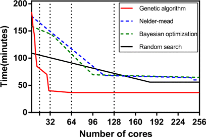
Fig. 3. Scaling of computational time for parallel execution of optimization techniques as the number of cores increases on linear.
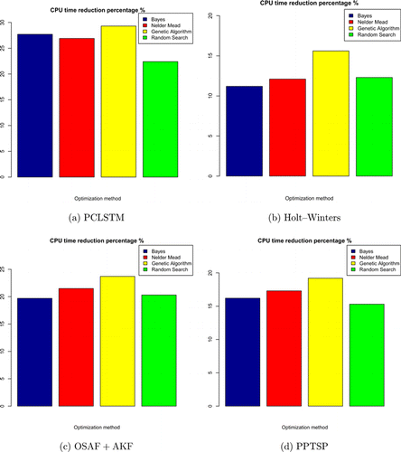
Fig. 4. CPU time reduction of the comparison methods with respect to the optimization methods. The results were recorded with the mainframe described in Sec. 5.3.
The analysis given in Figs. 6(a)–6(d) was performed to investigate whether the derivative-free optimization methods lead to overfitting or underfitting for PCLSTM. We can conclude that Bayesian optimization created an underfitting that two curves do not meet at any number of epochs. The genetic algorithm, which takes a very long time to complete training, resulted in overfitting.
Fluctuation properties of time series are generally examined to check whether there is a similarity among the experimental data. The knowledge acquired from that examination helps to establish training exploiting distinctive instances. To validate the distinctiveness of the training data sets, a correlation analysis was conducted. The analysis given in Fig. 5 shows that the training data of the experiment have dissimilar characteristics. However, the similarity between Natal and Manaus is not exact but tolerable. Manaus has two sharp changes in the time series. That case may have affected the increase in RMSE results given in Table 4. On the other hand, the minimum fluctuation was observed in PortoAlegre data set.
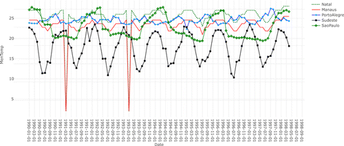
Fig. 5. Correlation analysis of the data sets.
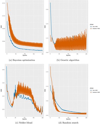
Fig. 6. Training versus Validation losses of optimization methods. Training curve was drawn with 70% of the data sets. Validation curve, on the other hand, denotes 15% of the all data sets.
To validate the superiority of PCLSTM over the other comparison methods, a nonparametric analysis namely the one-tailed Mann––Whitney U-test was performed by using the results presented in Table 4. PCSLTM was found to be significantly different from the baselines (p<0.05). An unpaired setting was used for each pair of columns.
Although Nelder–Mead was not able to yield lower RMSE than random search, it does not take much time compared to the genetic algorithm and random search. The actual and predicted lines of the prediction results are given in Figs. 7(a)–7(d). It is worth noting that Bayesian optimization yielded the worst result. Likewise, optimizing PCLSTM with Bayes resulted in underfitting. Moreover, using Bayes for hyperparameter optimization remarkably increased the RMSE, as given in Table 4. The best result was achieved with Nelder–Mead that leads to good fitting. Interestingly, the prediction performance of the random search is not similar to that of training. Instance selection is therefore of great importance for both training and testing when using random search. Further, there is a notable similarity between underfitting and optimization time. We know from preceding optimization studies that the Bayesian algorithm consumes more time than the genetic algorithm.63 Figure 6 validates that finding.
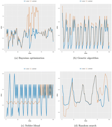
Fig. 7. The predicted results, which were obtained via PCLSTM, of randomly selected 100 sequential instances. The x-axis indicates index of the instance. Values of time series are graphed along the vertical axis.
The mainframe used in the experiment has 256 cores that are suitable for parallelization. Execution time and workload balance analyses are performed with that mainframe described in Sec. 5.3. Figures 7–9 show the time and workload balances of the comparison methods. In Fig. 8(a), the average execution times of the data sets are given in increasing number of nodes for PCLSTM. The workload balance decreases as the number of nodes increases regardless of the type of comparison algorithm but up to a specific threshold. The fall in line is very clear both for OSAF+AKF and PPTSP. On the other hand, the decline of workload in PCLSTM is lower than the competitive methods. The average execution time of Sudeste rapidly decreases up to 14 nodes. Since it has more than 9 million instances that are much more suitable for parallel execution. The workload balance of the mainframe is within the range of 0.78–0.71, as shown in Fig. 8(b). A stagnant range implies the most suitable number of cores for workload balance. Setting the number of nodes between 16 and 20 results in a consistent balance for the experiment. The workload balance is computed with64
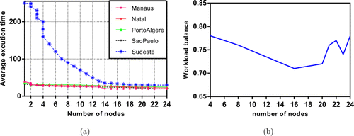
Fig. 8. Execution time (minutes): (a) and workload analysis, (b) of PCLSTM.
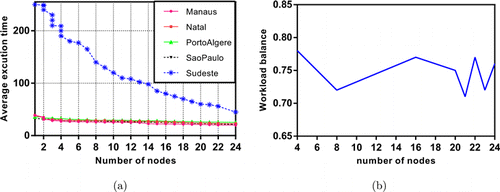
Fig. 9. Execution time (minutes) (a) and workload analysis, (b) of OSAF+AKF.
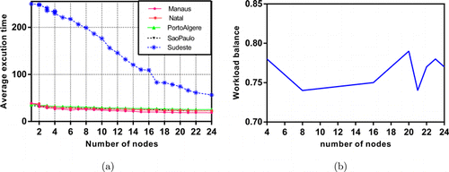
Fig. 10. Execution time (minutes) (a) and workload analysis, (b) of PPTSP.
7. Conclusion and Future Work
This paper investigates to what extent derivative-free optimization methods are beneficial in tuning parallel architecture designed for time series prediction. To that end, a new algorithm (PCLSTM) is devised by utilizing the fundamentals of LSTM. As a result, PCLSTM outperformed the other methods in RMSE. However, it requires a large number of instances to reduce prediction error as in the Sudeste data set. Parallelization established on PCLSTM resulted in the largest CPU time reduction (13%) on the genetic algorithm which takes a very long time on one core machine. To achieve a good fitting, Nelder–Mead needs a large number of iterations. On the other hand, the lowest prediction error was obtained via a random search. An improved version of this work may focus on the issues presented as follows:
| (1) | The method may be evaluated on a search technique such as differential evolution to extend the scope. | ||||
| (2) | PCLSTM was developed based on a classic LSTM. Instead, adopting other types of LSTM is an interesting point to investigate. | ||||
| (3) | This work is focused on tuning the hyperparameters of the LSTM. For this reason, the default hyperparameters of the derivative-search methods were employed in the experiment. We plan to develop a heuristic algorithm to initialize the hyperparameters of those methods. | ||||

