
Global Value Chains and Employment Growth in Asia
Abstract
This paper considers the sources of employment demand in Asian economies. Using data from the World–Input Output Database, I examine the relative importance of domestic and foreign demand in generating employment. Despite some degree of heterogeneity across the sample, domestic demand is found to be the major driver of employment in all cases. Further, the relative importance of final and intermediate exports in generating employment varies by economy, with some economies relying on intermediate exports to generate employment to a greater extent than others, reflecting their importance as suppliers of intermediate inputs in global value chains, while others rely to a greater extent on final exports, reflecting their role as assemblers within global value chains. Considering developments over time, I find that employment is driven by two offsetting factors: (i) final demand (either domestic or foreign) and (ii) labor productivity, with changes in interindustry structure also being important in the case of intermediate exports.
I. Introduction
International trade and the globalization of supply chains have been important drivers for the growth and development of a number of economies in Asia and beyond, most notably the People's Republic of China (PRC). Global value chains (GVCs) are often considered a relatively easy route to industrialization (Baldwin 2016). By enabling economies to contribute to certain stages of production, they avoid the problems associated with developing whole industries. In addition, GVCs are considered important channels for technology spillovers and technology upgrading. Despite concerns about potential negative consequences for workers (ILO 2011), there is also an expectation that GVC participation can promote employment in developing economies. With some notable exceptions (e.g., Los, Timmer, and de Vries 2015; Portella-Carbo 2016), however, there is a paucity of evidence on the impact of trade generally, and GVC participation in particular, on employment, both in absolute terms and relative to domestic sources of employment.
This issue of the relationship between trade and employment generation is even more relevant in the context of the recent global financial crisis that has been associated with weak and volatile demand in world markets. Indeed, there is evidence that levels of global trade and GVC participation have plateaued since the financial crisis and in recent years have actually declined (Timmer et al. 2016). A number of potential explanations for these recent developments in trade and GVC performance have been proposed: weak demand in response to the crisis; the lack of progress in multilateral and bilateral trade policy negotiations—in particular with regard to standards, regulations, and rules of origin, among others—that have limited further fragmentation; the possibility of overfragmentation that is now being corrected; an increase in the extent of reshoring; and the possibility that the benefits of major technological developments, particularly in information and communication technology, have been exhausted.
In this paper, I am interested in identifying recent (2000–2014) developments in employment in a sample of six Asian economies and decomposing these developments along a number of dimensions. In particular, I decompose employment developments into effects due to domestic and foreign demand, where this latter effect is further split into effects due to foreign final demand (final exports) and foreign intermediate demand (intermediate exports). I use a structural decomposition analysis to decompose employment growth in the sample of economies into effects due to labor productivity growth, final demand growth, changes in interindustry structure, and changes in the ratio of value-added growth.1 Finally, I identify differences in employment growth and the drivers of employment growth between the precrisis and postcrisis periods.
The analysis is linked to a number of different strands of literature. It is linked, for example, to the small existing literature on measuring the employment effect of exporting.2 A number of these papers consider this relationship in the context of the PRC, with Feenstra and Hong (2010) using input–output analysis to estimate the employment effects of exporting. They find that export growth contributed around a third of overall employment growth during 1997–2005, with most growth coming from nontraded goods like construction. While exports grew much faster during 2000–2005, developments in domestic demand continued to dominate. Similar results were found by Chen et al. (2012), who show that the impact on employment of processing exports was lower than that of nonprocessing exports, which in turn was significantly lower than the effect due to domestic demand. Los, Timmer, and de Vries (2015) adopt a similar approach to identify the direct and indirect employment effects of exports in the PRC. Their results indicate that between 1995 and 2001, rapid growth in foreign demand was offset by large increases in labor productivity, with the result being that foreign demand had essentially no effect on net employment. During 2001–2006, however, a strong rise in foreign demand resulted in about 70 million jobs being added. In the most recent period for which data were available (2006–2009), domestic demand became more important than foreign demand, which the authors argue may signal a rebalancing of the global economy.
Other studies conduct similar analyses for different economies. Feenstra and Sasahara (2017), for example, estimate the impact on employment in the United States (US) from exports and imports during 1995–2011. They find that growth in US exports led to increased demand for workers that generated around 6.6 million new jobs. Imports into the US from the PRC reduced labor demand by about 2 million jobs, which still resulted in an overall net gain for the US during the review period in terms of employment demand from importing and exporting. Kiyota (2014) considers the impact of exports on employment in the cases of the PRC, Indonesia, Japan, and the Republic of Korea, with the results indicating a positive and increasing effect of exports on employment in Japan, the PRC, and the Republic of Korea. The study further shows the important role of machinery-related industries in generating employment through exports, with indirect employment effects through vertical interindustry linkages also playing an important role.
In a recent paper, Portella-Carbo (2016) extends this kind of analysis to consider the super-multiplier effects of international trade. In his model, trade impacts employment in a manner similar to the studies mentioned above, but has additional impacts by stimulating household consumption, private business investment, and the production of intermediate goods. In short, autonomous demand impacts employment through the Keynesian multiplier and the accelerator mechanism. His results indicate that the effects of trade on employment vary greatly across economies, with the effects in upswings being particularly large in economies such as the PRC and Germany, but smaller in other economies such as France and the United Kingdom, which rely to a greater extent on domestic demand.
The current paper is also linked to recent work on the effects of the crisis on trade patterns. Timmer et al. (2016) consider the decline in world trade in the postcrisis period, arguing that there are two competing explanations for the changed circumstances. The first is that the composition of demand has changed, in particular from durable investment and consumer goods toward services that are less trade intensive (Bems, Johnson, and Yi 2011, 2013; and Bussière et al. 2013). The second relates to the possible decline of GVC activity that may have occurred for a number of reasons already mentioned above (Evenett and Fritz 2015; Kee and Tang 2016; Harms, Lorz, and Urban 2012). Timmer et al. (2016) find that both channels have played a role in the stalled development of international trade. My analysis of the precrisis and postcrisis periods in this study's dataset extends the analysis of Timmer et al. (2016) to consider the employment implications of changes in international trade activity.
The starting point for the approach that I adopt in this paper is the analysis of Los, Timmer, and de Vries (2015), who consider the impact of foreign demand on employment creation in the PRC. The approach builds upon recent applications of input–output tables to issues of international trade (Timmer et al. 2013, 2014; Foster-McGregor and Stehrer 2013; Koopman, Wang, and Wei 2014; Wang et al. 2017) by estimating the consequences of developments in international trade for domestic employment. The analysis is based upon the recently released update to the World Input–Output Database (WIOD) (Timmer et al. 2015), which has data from 2000 to 2014. I concentrate on the six Asian economies included in the WIOD: India; Indonesia; Japan; the PRC; the Republic of Korea; and Taipei,China.
The main interest of the analysis is to identify to what extent the crisis has impacted labor demand and whether there has been a shift away from foreign demand toward domestic demand. At the same time, there are a number of additional hypotheses that are implicit in the analysis. In particular, I expect that the smaller economies in the sample are reliant to a larger extent on exports for generating labor demand than larger economies, which in turn are likely to have a more diversified production structure. As such, the smaller economies in the sample may be affected to a greater extent in the postcrisis period by the observed declines in trade and GVC activity. In addition, theory indicates that changes in the terms of trade between primary products and manufactures will affect natural resource-poor economies in the opposite way as resource-rich economies such as Indonesia. The period 2000–2014 was one in which the terms of trade improved dramatically for resource-rich economies such as Indonesia and deteriorated substantially for the other five Asian economies in the sample. As such, I may expect that the resultant real exchange rate changes would favor growth in the demand for nontradables—and as a result the demand for domestic goods—in Indonesia, with the opposite being the case in the other five sample economies.
The results of the analysis indicate that domestic demand is the major driver of employment in all six economies, albeit to a lesser extent in some economies. The relative importance of final and intermediate exports in generating employment also varies by economy. Some economies such as Taipei,China rely on intermediate exports to generate employment to a greater extent than others, likely reflecting their importance as suppliers of intermediate inputs in GVCs. Other economies such as the PRC rely to a greater extent on final exports, reflecting their role as assemblers within GVCs. Considering developments over time, I find that employment is driven by two offsetting factors: (i) final demand (either domestic or foreign) and (ii) labor productivity. In the case of intermediate exports, changes in interindustry structure have also played a role in many economies.
The remainder of the paper is set out as follows. Section II describes the methodology used in the analysis. Section III briefly discusses the data. Section IV presents the results. Section V concludes.
II. Methodology
The initial approach to identify the employment effects of international trade and GVCs follows closely that adopted by Los, Timmer, and de Vries (2015), which in turn was based upon the contribution of Johnson and Noguera (2012). Here, the approach of Los, Timmer, and de Vries (2015) is described in detail before discussing the extension of this approach.
I begin by assuming that there are N economies, S industries in each economy, and F production factors in each economy–industry. Industry output in a particular economy is determined using domestic production factors, in this case capital and labor, and intermediate inputs, which may be sourced either domestically or from foreign sources. The output produced in each industry can be used as either final demand or as intermediate inputs in the production of other goods. Demand for final goods is assumed to come from three sources: (i) households, (ii) government, and (iii) firms.3 When considering shipments of final goods and intermediates, both within and across economies, there needs to be a distinction between the source and destination economy–industry. Following Los, Timmer, and de Vries (2015), I use i to denote the source economy, j the destination economy, s the source industry, and t the destination industry. It is assumed that markets clear and the additional assumption of a single price irrespective of a product's use is imposed. By definition, when markets clear, the product-market-clearing condition can be written as
Here, yi(s) is the value of output in industry s in economy i, fij(s) is the value of goods sold by this industry for final use in economy j, and mij(s,t) is the value of products sold by this industry for intermediate use by industry t in economy j.
Los, Timmer, and de Vries (2015) go on to express the market-clearing conditions for each of the SN industries using matrix algebra. To do this, let y be the output vector of dimension (SN×1), the elements of which represent output levels in each economy–industry. A global input–output matrix A of dimension (SN×SN) is also defined. The matrix has elements aij(s,t)=mij(s,t)/yj(t), which capture the ratio of intermediate inputs per unit of output and are termed the technical coefficients. Los, Timmer, and de Vries (2015) describe these terms as giving the cost shares of output from industry s in economy i used by industry t in economy j. The matrix A can be written as
Using the matrix A, equation (1) can be expressed in matrix form as
To complete their model, Los, Timmer, and de Vries (2015) assume that the quantity of output in an industry is a function of the quantities of the labor, capital, and intermediate inputs used in production. The value of output in an industry is then equal to the value of all inputs used. Denoting the value of output in industry s of economy i as yi(s), and letting li(s) denote the number of workers in this industry, I can then define pi(s) as the number of workers required per US dollar of output in industry s in economy i:
Equation (4) is the main equation of interest in capturing the importance of final demand for employment generation. I extend this approach in two ways. Firstly, I use the recent approach of Wang et al. (2017) to further decompose the sources of employment generation. Secondly, I use a structural decomposition approach to identify the sources of recent developments in employment generation.
The approach of Wang et al. (2017) decomposes production activities into three terms: (i) production for domestic demand, (ii) final goods exports, and (iii) intermediate exports (what they term GVC activities and which may also involve the reimportation of intermediates at later stages of the production process). The approach of Wang et al. (2017) begins by rewriting equation (2) as
Rearranging equation (5) gives
This equation decomposes the labor used in each economy–industry into the following:
| (i) | Employment generated domestically for domestic final demand (ˆpLfD) | ||||
| (ii) | Employment generated domestically for final production exports (ˆpLfF) (i.e., employment generated for production that crosses borders for final consumption only) | ||||
| (iii) | Employment generated through the export of intermediate goods (ˆpLAFBf) | ||||
Equation (6) indicates that labor induced through these different channels of demand depends upon three sets of factors: (i) changes in labor requirements (ˆp); (ii) changes in the intermediate input structure (L,B,andAF); and (iii) changes in the level of final demand (f,fD,andfF). For ease of exposition, I can rewrite equation (6) as
The description above is based closely upon that provided by Los, Timmer, and de Vries (2015) and has been extended to introduce the approach of Wang et al. (2017). Within this framework, I now use the time series that I have available to decompose the growth in employment due to final demand. To do this, I begin by noting that 1 plus the growth rate of employment between two time periods (0 and 1) (or the ratio of employment due to final demand) can be expressed as follows:
Using standard decomposition methods, it is possible to decompose this expression into an effect due to changes in (i) employment to gross output (i.e., employment requirements); (ii) interindustry structure, both domestically and internationally); and (iii) foreign final demand. The resulting decomposition is as follows:
This expression can be further decomposed to capture the role of labor productivity changes in driving employment changes. To see this, the standard definition of labor productivity (i.e., value added per worker) can be written as
This states that the ratio of employment to gross output is equal to the inverse of labor productivity multiplied by the ratio of value added to gross output. Substituting equation (10) into equation (8) gives
The first term captures the impact of changing labor productivity on employment, the second captures the impact of changing value added to gross output ratios, the third captures the impact of changes in technical coefficients (i.e., intermediate use), and the final term captures changes in foreign final demand. This is the final decomposition of overall employment demand. Note, however, that the approximate growth rate of employment (due to foreign demand) between two time periods can be written as
| (i) | an effect due to changes in labor productivity (q); | ||||
| (ii) | an effect due to changes in the ratio of value added to gross output (w), which is often considered to be driven by upgrading within GVCs; | ||||
| (iii) | an effect due to changes in the interindustry structure (B), including the role of a changing trade structure in intermediate goods, that may be due to such things as factor substitution, technological change, and (GVC) sourcing patterns; and | ||||
| (iv) | an effect due to changes in final demand. | ||||
The studies of Feenstra and Hong (2010) and Chen et al. (2012) mentioned above argued that the employment impact of (foreign) demand growth crucially depend on the levels and growth rates of the labor productivity of the various activities. In particular, they argue that the employment effect of foreign demand is mainly a race between increases in productivity levels and demand levels, with higher productivity reducing the induced demand for labor (holding foreign demand constant). The decomposition defined above allows this hypothesis to be addressed in a more formal way.
A similar decomposition can be written for the individual terms of equation (7) as follows:
Note that equation (14) includes additional terms capturing the effects of AF (the imported input coefficients) and B (the full Leontief matrix). While I do calculate the full decomposition in this case, the results combine the three terms capturing the interindustry structure (L,AF,andB), which allows for a ready comparison with the results from the other decompositions. In addition, foreign final demand can be further decomposed by the source of that demand. In the analysis that follows, I decompose foreign final demand across four regions—Asia, the Americas, Europe, and the rest of the world—to examine the regional sources of employment growth in Asia.
III. Data and Descriptive Statistics
The analysis is conducted using the 2016 version of the WIOD, which builds upon and extends the 2013 version of the dataset.4 WIOD constructs a world input–output table for 43 economies (plus the rest of the world) for the period 2000–2014 and includes data on 56 sectors, mainly at the 2-digit ISIC Revision 4 level (see Timmer et al. [2015, 2016] for details on construction and coverage). In addition to world input–output tables, WIOD also reports a set of socioeconomic accounts that include information on employment levels (in terms of both hours worked and persons engaged).
The WIOD therefore has all the relevant information needed to conduct the analysis that follows. I make use of (i) the international input–output tables (reporting the values of intermediate flows between all industries and economies), (ii) value added by economy and industry, (iii) gross output by economy and industry, (iv) domestic and foreign final demand by economy and industry, and (v) employment by economy and industry.5 In this analysis, I am forced to measure employment in thousands of workers rather than hours worked. This is largely because data on hours worked are not available for the PRC.
The time series of world input–output tables on which the empirical analysis is based are expressed in current US dollars. Given the interest in developments over time, this creates an issue when variables are expressed as ratios of quantities (e.g., number of employees) to values (e.g., the value of gross output). To deal with this, I follow the approach of Los, Timmer, and de Vries (2015) and deflate all nominal values using the gross domestic product deflator from the World Development Indicators database.
IV. Results
A. Employment Developments in Asia
In this subsection, I present initial descriptive results, describing developments in employment generation in Asian economies over the period 2000–2014 and the sources of demand for this employment.
Table 1 presents the initial level of employment in 2000 for the six sample economies, along with the decomposition of employment given by equation (5) into employment due to domestic demand and the two sources of foreign demand (final exports and intermediate exports). The table shows that employment in 2000 was around 720 million and 410 million in the two economies with the largest populations, the PRC and India, respectively. The two smallest economies in population terms, Taipei,China and the Republic of Korea, had employment levels in 2000 of around 17 million and 18 million, respectively. Domestic consumption accounted for the vast majority of employment in all of the sample economies, being as high as 91% in India and Japan, with lower levels reported in the Republic of Korea (80%); Indonesia (79%); and Taipei,China (74%).6 The fact that these latter economies rely to a greater extent on trade for their labor demand may reflect the fact that they are relatively small in terms of gross domestic product and are therefore generally more open to trade. Among trade channels, final exports accounted for the greatest share of employment in the PRC and India, possibly indicating the importance of assembly activities for the PRC in particular. Intermediate exports accounted for the greatest share in the other four economies, with the difference between employment due to intermediate and final exports being relatively large in Taipei,China.
| Employment Due To: | ||||
|---|---|---|---|---|
| Economy | Employment | Domestic Consumption | Final Exports | Intermediate Exports |
| India | 410.1 | 372.9 | 19.8 | 17.5 |
| 91% | 5% | 4% | ||
| Indonesia | 96.9 | 76.3 | 8.6 | 12.0 |
| 79% | 9% | 12% | ||
| Japan | 65.3 | 59.5 | 2.6 | 3.1 |
| 91% | 4% | 5% | ||
| PRC | 719.6 | 620.5 | 57.8 | 41.3 |
| 86% | 8% | 6% | ||
| Republic of Korea | 18.2 | 14.6 | 1.7 | 2.0 |
| 80% | 9% | 11% | ||
| Taipei,China | 16.9 | 12.6 | 1.8 | 2.6 |
| 74% | 11% | 16% | ||
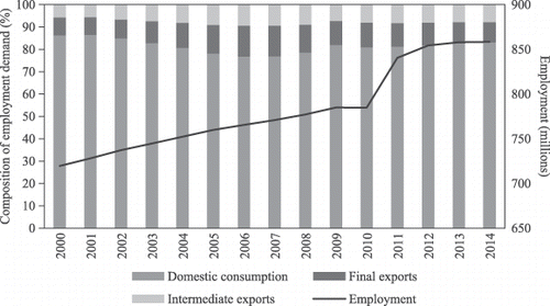
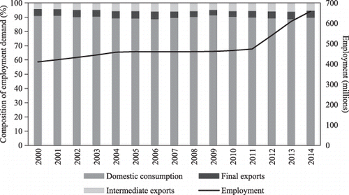
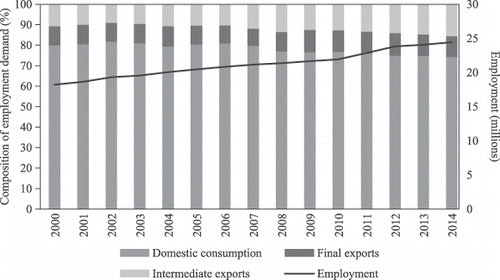
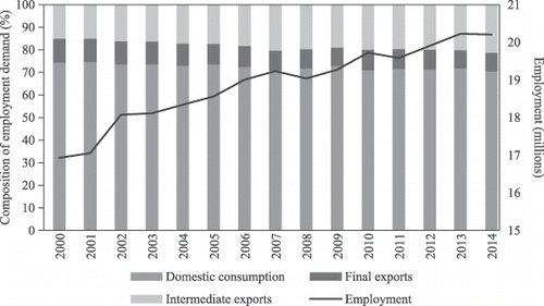
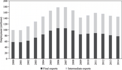
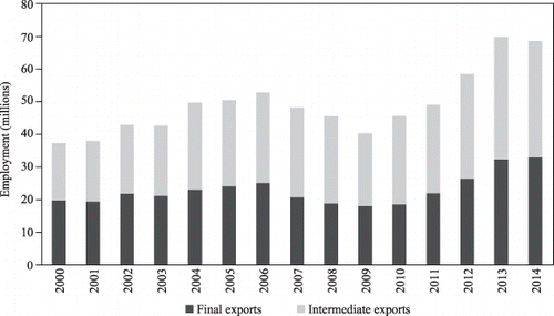
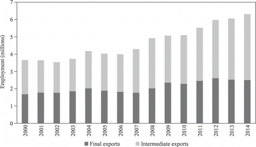
Figures 1.1–1.6 report employment levels for each of the six economies over the full review period (2000–2014), as well as the decomposition of employment into three sources (domestic consumption, final exports, intermediate exports). Considering each economy in turn, Figure 1.1 shows that employment in the PRC rose steadily during the review period, despite a small decline around the time of the global financial crisis, with a notable increase in employment during 2010–2011. The role of domestic demand dropped somewhat during the early 2000s, but increased after the financial crisis. This may be related to a general reorientation of the PRC's economy toward domestic demand. The declining share of domestic demand in generating employment in the early 2000s was offset by a rising share of both forms of exports, with demand due to final exports rising to a larger extent than demand due to intermediate exports. In the case of Indonesia, Figure 1.2 shows increasing employment, with a relatively rapid rise after 2011. Unlike the PRC, there was no observed decline in employment around the time of the financial crisis. Also, in contrast to the PRC, there is a rising share of domestic final consumption in employment generation across the whole review period, with declining contributions of both final exports and intermediate exports over time. This provides some support to the view expressed above that developments in the terms of trade may have led to increased demand for nontradables in relatively resource-rich Indonesia. The results for India in Figure 1.3 also confirm a positive employment trend, with a noticeable increase after 2011. In general, there is little in the way of changes in the composition of employment sources.
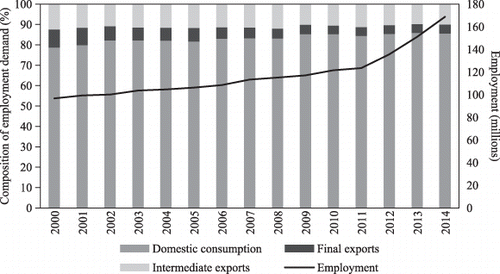
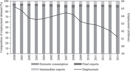
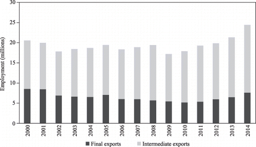
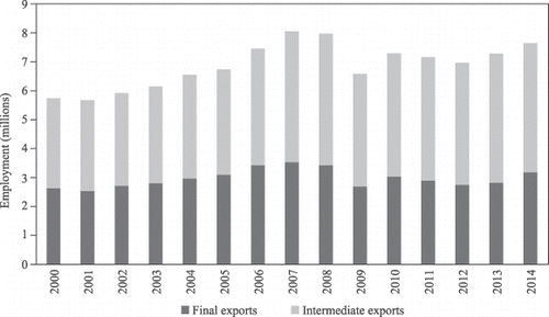
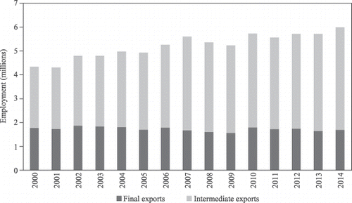
In the case of Japan, Figure 1.4 shows a different pattern of generally declining employment, which was more pronounced after the global financial crisis. In terms of the sources of employment demand, there was a slight decline in the role of domestic consumption over time, with small increases in the role of all trade activities. Developments in the Republic of Korea, as shown in Figure 1.5, fit with the pattern found for all sample economies other than Japan, with a rising trend in employment demand. The importance of domestic consumption for employment generation tended to decline over time, with a rising share of employment demand for the two forms of exports, particularly intermediate exports, observed. The results for Taipei,China in Figure 1.6 largely mimic those for the Republic of Korea, with a rising trend in employment demand and a declining role for domestic consumption in generating this demand during the review period.
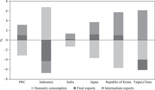
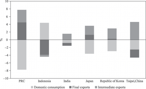
To emphasize changes in the contributions of the different sources of employment demand over time, Figure 2 reports changes (in percentage points) in the different sources of employment demand for the six sample economies between 2000 and 2014. In most economies, the share of domestic consumption in generating employment declined during the review period. The only exception to this was Indonesia where the share of employment due to domestic consumption increased by nearly 7 percentage points, with both forms of international trade seeing a declining share, most notably final exports. In the other economies, a declining share of domestic consumption was observed, with declines ranging from a low of around 1.5 percentage points in India to a high of nearly 6 percentage points in the Republic of Korea. In all of these cases, the contributions of both trade channels tended to increase, with the exception of Taipei,China for final exports, where employment due to intermediate exports accounted for much of the increase.
PRC = People's Republic of China.
B. Decomposition Results
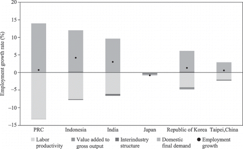
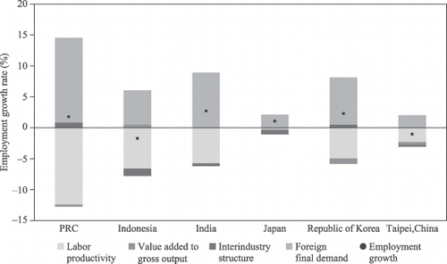
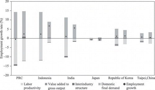
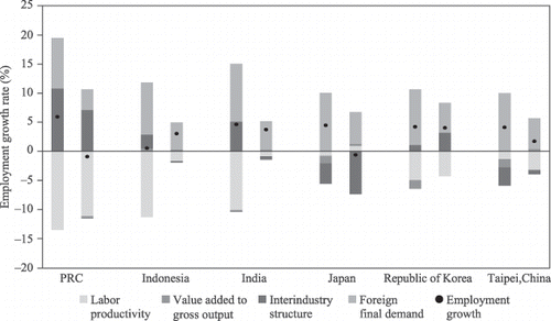
The previous subsection described developments in employment demand and the sources of this demand. This subsection reports results from decomposing the different sources of employment demand as shown in equations (12), (13), and (14).7 Figure 3 shows the average annual growth rate of employment during 2000–2014 due to domestic final demand, along with the decomposition of this growth. In most economies, the average growth rate of employment due to domestic final demand was low, and even negative in the case of Japan. The exceptions to this were Indonesia and India, which reported average growth rates of employment due to domestic final demand of 4.2% and 3%, respectively. In terms of the decomposition of employment growth, I tended to find a relatively large positive effect of domestic final demand and a relatively large negative effect of labor productivity growth. In the PRC, the Republic of Korea, and Taipei,China, these two effects tended to offset each other, resulting in a muted effect of domestic final demand on employment growth. In Indonesia and India, the growth in domestic final demand was higher than the growth in labor productivity during the review period, resulting in relatively strong employment growth. The final case of Japan is interesting, with essentially no growth in either domestic final demand or labor productivity during 2000–2014. The other thing to note from this figure is the almost complete lack of a role for either the growth in the ratio of value added to gross output or the interindustry trade structure.
PRC = People's Republic of China.
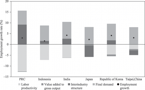
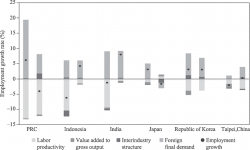
Figures 4 and 5 report information on employment growth due to the two forms of international trade, final exports and intermediate exports, along with the corresponding decomposition of these effects. Considering final export demand (Figure 4), relatively low growth rates of employment due to final export demand are again observed. The growth effects range from a low of –1.7% in Indonesia to a high of 2.7% in India. Once again, the overall effects are driven by the (offsetting) growth effects of final demand and labor productivity, with the effects of changes in the interindustry structure and the growth rate of value added to gross output being generally small. Despite similar and muted growth effects, there are important differences across the sample economies. In the case of the PRC, the growth of foreign final demand was relatively high (around 14%), with relatively high growth rates also being observed in India (8.9%) and the Republic of Korea (7.6%). Labor productivity growth in these economies was also relatively high, however, leading to a small overall growth effect. In other economies, most notably Japan and Taipei,China, the growth of foreign final demand was relatively low at around 2%.
PRC = People's Republic of China.
PRC = People's Republic of China.
Turning to the case of intermediate exports and their impact on employment growth (Figure 5), somewhat similar results are observed.8 Firstly, employment growth due to intermediate exports tends to be higher than the rates observed for the case of foreign final demand. Growth rates range from 1.6% (Indonesia) to 4.2% (India). Secondly, final demand is usually the main driver of employment growth due to intermediate exports, with the growth effects of final demand ranging between 6.5% and 8.1%. Thirdly, labor productivity growth has a strong (negative) impact on employment growth due to intermediate exports across economies, with the main exception being Japan, where labor productivity growth has been muted, and to a lesser extent Taipei,China. Fourthly, and unlike the previous cases, changes in the interindustry structure play an important role in driving employment growth due to intermediate exports in a number of economies. The most important example in this context is the PRC, where the effect of interindustry structure is large and dominates the effect of final demand. This suggests that in the PRC, developments in sourcing patterns have strongly impacted employment growth due to GVC participation. This may indicate the movement from a reliance on upstream intermediate imports to an increasing reliance on domestic upstream intermediate inputs in the PRC. Changes in interindustry structure also impacted positively upon employment growth in India, Indonesia, and the Republic of Korea. Negative effects were observed in the cases of Japan and Taipei,China, with changes in sourcing patterns reducing employment growth in both of these economies.
C. Precrisis and Postcrisis Developments in Employment
The previous subsection showed that of the different forms of international trade considered, the employment effects of intermediate exports tended to grow more rapidly during 2000–2014. This subsection considers whether there were differences in employment developments (and the corresponding decompositions) between the precrisis and postcrisis periods. As already discussed, developments in trade flows and GVC participation tended to differ in the precrisis and postcrisis periods, with this subsection examining whether there have been similar effects on employment.
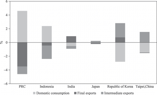
Figures 6 and 7 report results that are similar to Figure 2 but for the two subperiods, 2000–2008 and 2009–2014, respectively.9 Changes in the composition of employment demand tended to be larger during 2000–2008 than 2009–2014. During the former period, results indicate that employment demand due to international trade tended to increase relative to demand due to domestic consumption. This was true for all cases except Indonesia. In most economies, the rise in employment demand resulting from international trade was due largely to intermediate exports, with the effect of final exports being negative for India; Indonesia; and Taipei,China. The major exception was the PRC, where demand due to final exports was dominant.
PRC = People's Republic of China.
PRC = People's Republic of China.
While smaller than during 2000–2008, the changing composition of employment demand during 2009–2014 followed a similar pattern in the Republic of Korea and Taipei,China, with an increasing contribution of intermediate exports at the expense of domestic consumption. In the PRC, there was a change in the relative roles of international trade and domestic consumption, with the role of domestic consumption increasing and the role of international trade, most notably final exports, falling. The pattern in Indonesia during 2009–2014 was similar to that during 2000–2008, albeit with intermediate exports accounting for most of the decline in the contribution of international trade. In India and Japan, the overall changes and the changes in composition were relatively small.
Table 2 reports the average growth rates of employment for three different demand sources during 2001–2008 and 2009–2014. The table reveals a number of interesting outcomes. In a number of economies, the growth rate of employment generation in the postcrisis period actually exceeded that in the precrisis period for all three sources of demand. This is true for Indonesia and India, and, except in the case of intermediate exports, also for the Republic of Korea. For two of these economies—Indonesia and India—employment growth due to final exports was actually negative in the precrisis period. In the cases of the PRC and Japan, there is negative employment growth due to final exports in the postcrisis period, following relatively rapid growth in the precrisis period, with a small negative growth rate of employment for Japan (−0.5%) and a larger negative effect for the PRC (−3.5%). For these two economies, a similar pattern is also observed in the case of intermediate exports, with a small negative growth rate of employment in the postcrisis period after experiencing relatively rapid growth in the precrisis period. For the PRC, this relatively poor performance in the postcrisis period is offset by relatively rapid employment growth due to domestic consumption; while in the case of Japan, employment demand due to domestic consumption was also sluggish.
| Domestic Consumption | Final Exports | Intermediate Exports | ||||
|---|---|---|---|---|---|---|
| 2001–2008 | 2009–2014 | 2001–2008 | 2009–2014 | 2001–2008 | 2009–2014 | |
| India | 1.34 | 6.20 | −0.17 | 10.28 | 5.78 | 5.89 |
| Indonesia | 2.89 | 7.18 | −4.62 | 5.23 | 1.77 | 3.88 |
| Japan | −0.70 | −0.80 | 3.45 | −0.47 | 4.95 | −0.01 |
| PRC | −0.20 | 2.68 | 7.10 | −3.54 | 7.00 | −0.10 |
| Republic of Korea | 1.57 | 1.64 | 2.59 | 3.81 | 5.23 | 4.84 |
| Taipei,China | 1.05 | 0.66 | −1.16 | 1.09 | 5.08 | 2.33 |
Given the interest in the effect of the crisis on employment and the channels of employment generation, Figures 8.1–8.6 report the employment generated by international trade for each of the six economies during 2000–2014. Considering each economy in turn, Figure 8.1 shows that in the PRC, employment due to international trade dropped dramatically around the time of the crisis. Between 2008 and 2009, employment due to foreign demand dropped 14.9%, following a drop of about 6% between 2007 and 2008. The decline was driven by changing demand due to both final and intermediate exports, with a somewhat larger percentage decline in employment demand due to intermediate exports. However, the recovery in employment following the crisis also tended to be more rapid in the case of intermediate exports. Figure 8.2 shows that in Indonesia, there was a more prolonged drop in employment due to final exports, though at the time of the crisis, the percentage decline in demand due to intermediate exports was much stronger (though, as with the PRC, it also recovered more quickly). This was also the case with India, as shown in Figure 8.3, which saw relatively large percentage declines in employment demand due to final exports in the lead-up to the crisis and a large drop in demand due to intermediate exports at the time of the crisis during 2008–2009. Figure 8.4 shows that the case of Japan is somewhat different, with the decline in demand at the time of the crisis due to final exports being significantly larger than that due to intermediate exports. The recovery in Japan was also slower, with levels of employment due to final exports and intermediate exports not having reached their precrisis levels by 2014. The Republic of Korea also exhibited a pattern dissimilar to some of the other economies. Figure 8.5 shows rising employment demand due to final exports continuing to grow throughout the crisis alongside a relatively minor contraction in employment due to intermediate exports. Results thus suggest that the Republic of Korea was largely shielded from the effects of the crisis, at least in terms of the employment impact of foreign demand. The negative impacts of the crisis on employment demand were also relatively muted in the case of Taipei,China. Figure 8.6 shows the declines in demand being fairly evenly split between final and intermediate exports.
The final part of this subsection reports the decomposition results for the precrisis and postcrisis periods separately. The decomposition results are reported for domestic consumption in Figure 9, for final exports in Figure 10, and for intermediate exports in Figure 11. In these figures, the left-hand side of each pair of bars for each economy reports the decomposition for the precrisis period (2001–2008) and the right-hand side bars are for the postcrisis period (2009–2014).
I begin with the decomposition of employment growth due to domestic final demand. Figure 9 reveals that employment growth due to domestic demand tended to be higher in the postcrisis period than in the precrisis period. The difference in growth rates between the two periods was particularly large in the case of Indonesia (2.3% versus 6.7%) and India (1.1% versus 5.6%). Decomposition results indicate largely offsetting effects of domestic demand growth and labor productivity growth, with only small effects of either changes in interindustry structure or the ratio of value added to gross output. The majority of cases show a declining role for labor productivity growth in the postcrisis period, with the difference between the precrisis and postcrisis periods being particularly large in the case of Indonesia and India. The role of domestic demand growth in the postcrisis period also declined in many of the sampled economies—and became negative in the case of Japan—with a slight increase in the contribution of domestic demand growth observed only in Taipei,China.
PRC = People's Republic of China.
Note: The precrisis period refers to 2001–2008, while the postcrisis period refers to 2009–2014.
PRC = People's Republic of China.
Note: The precrisis period refers to 2001–2008, while the postcrisis period refers to 2009–2014.
PRC = People's Republic of China.
Note: The precrisis period refers to 2001–2008, while the postcrisis period refers to 2009–2014.
Turning to the trade channels, Figures 10 and 11 reveal that the (negative) effect of labor productivity on employment growth diminished in most economies (most notably Indonesia and India) in the postcrisis period relative to the precrisis period, with declines in labor productivity increasing employment in the case of Japan (implying a reduction in labor productivity). The (positive) effect of final demand growth also tended to decline in the postcrisis period relative to the precrisis period. This is particularly the case for employment growth due to intermediate exports (Figure 11), with large changes in the case of final exports limited to the PRC and Japan (Figure 10). In the case of intermediate exports, there was an important role for changes in the interindustry structure in many economies, most notably the PRC and Japan. Comparing the precrisis and postcrisis periods, changes in interindustry structure tended to lead to a decline in employment growth in the postcrisis period. This is true for all of the sample economies except the Republic of Korea and Taipei,China.
V. Conclusion
There is evidence of declining engagement in GVCs since 2008 at the global level, as well as for a number of Asian economies, most notably the PRC; the Republic of Korea; and Taipei,China. This paper considers the employment implications of these developments. While it is difficult to generalize across the diverse set of Asian economies considered, the results suggest that despite declining trade and GVC participation, growth in employment demand has been stable, and in some cases has increased, since 2008. Domestic demand accounts for the vast majority of employment demand, though effects differ by economy. Domestic demand is found to be relatively less important in the Republic of Korea and Taipei,China, possibly reflecting their relatively small size, and it has declined in importance for a number of economies in the postcrisis period. The case of the PRC is particularly interesting and suggests a reorientation toward domestic sources of demand. Indonesia is also relying increasingly on domestic sources of demand, possibly driven by global and regional terms of trade developments. Such results may raise questions about the overall importance of GVC involvement for employment, though the employment (and incomes) generated through foreign final demand may have relatively large multiplier effects, indirectly impacting employment through domestic demand.
In terms of the role of trade in generating employment, results differ by economy. Some economies rely on intermediate exports to generate employment to a greater extent than others, reflecting their importance as suppliers of intermediate inputs (e.g., Taipei,China) or raw materials and primary products (e.g., Indonesia). Others, most notably the PRC, generate more employment through final exports, reflecting their role as assemblers within GVCs. Developments in employment tend to be driven by two offsetting factors: (i) final demand (either domestic or foreign) and (ii) labor productivity. The positive role of final demand and changes in interindustry structure have tended to more than offset the negative effects of labor productivity growth. In the case of intermediate exports, changes in interindustry structure have also played a role in many economies, suggesting that there has been a reorientation in supply chains that have impacted employment positively in some economies (e.g., the PRC) and negatively in others (e.g., Japan). Since the global financial crisis, developments in interindustry structure have in general tended to impact negatively upon employment growth relative to the precrisis period.
The importance of foreign demand for employment growth has diminished for most economies since 2008. This has been offset by weaker labor productivity growth in the postcrisis period for most economies, which has minimized the effect of weak foreign demand on employment growth. As such, and despite the weak foreign demand growth, the declines in labor productivity growth have resulted in an increased growth rate of employment due to foreign demand in economies such as India and Taipei,China (in the case of final demand).
Notes
1 This study includes ex post analysis and does not identify the cause of changes in labor productivity or final demand, which are exogenously given.
2 The analysis is also linked to the literature estimating econometrically the relationship between offshoring and employment (e.g., Hijzen and Swaim 2010; Foster-McGregor, Poeschl, and Stehrer 2016). In these studies, offshoring is considered to have two offsetting effects: (i) a substitution effect that leads to the destruction of jobs, and (ii) a productivity effect that increases overall output and impacts positively upon employment. The approach adopted in these studies is to identify the overall effect of offshoring on employment, with a positive (negative) effect being interpreted as implying that the productivity effect is stronger (weaker) than the substitution effect. In the decomposition in section IV.B, I split up the effects of labor productivity and final demand, isolating the effects of each of these variables on employment demand.
3 In the WIOD 2016 release, final demand is split into five sources: (i) final consumption expenditure by households, (ii) final consumption expenditure by nonprofit organizations serving households, (iii) final consumption expenditure by government, (iv) gross fixed capital formation, and (v) changes in inventories and valuables.
4 The major drawback of the 2016 version compared with the 2013 version is the lack of information on employment by skill type, which thus does not allow for an analysis of the changing role of demand on employment composition.
5 The sources for data on employment, which can be found in Gouma et al. (2018), are varied and do not always coincide with official national data.
6 This study only accounts for the direct effect of the different trade channels on employment. The adopted approach is not able to account for indirect effects on employment through increases in the incomes of workers and firms that can raise domestic demand and demand for employment through increased household consumption and firm investment.
7 The decomposition as described above decomposes employment growth at the economy-sector level. In order to aggregate up to the economy level, sectoral employment weights are used in equations (12), (13), and (14).
8 As discussed above, the three terms that capture the effects of changes in interindustry structure—broadly defined—are combined in order to provide a ready comparison with the other two decompositions.
9 Average growth rates are reported for the periods 2000–2008 and 2009–2014, implying that the growth rate of 2009 includes information on employment levels in 2008. Using 2007 as the cutoff year rather than 2008 does not alter the qualitative results significantly.

