DecodeSTORM: A user-friendly ImageJ plug-in for quantitative data analysis in single-molecule localization microscopy
Abstract
Quantitative data analysis in single-molecule localization microscopy (SMLM) is crucial for studying cellular functions at the biomolecular level. In the past decade, several quantitative methods were developed for analyzing SMLM data; however, imaging artifacts in SMLM experiments reduce the accuracy of these methods, and these methods were seldom designed as user-friendly tools. Researchers are now trying to overcome these difficulties by developing easy-to-use SMLM data analysis software for certain image analysis tasks. But, this kind of software did not pay sufficient attention to the impact of imaging artifacts on the analysis accuracy, and usually contained only one type of analysis task. Therefore, users are still facing difficulties when they want to have the combined use of different types of analysis methods according to the characteristics of their data and their own needs. In this paper, we report an ImageJ plug-in called DecodeSTORM, which not only has a simple GUI for human–computer interaction, but also combines artifact correction with several quantitative analysis methods. DecodeSTORM includes format conversion, channel registration, artifact correction (drift correction and localization filtering), quantitative analysis (segmentation and clustering, spatial distribution statistics and colocalization) and visualization. Importantly, these data analysis methods can be combined freely, thus improving the accuracy of quantitative analysis and allowing users to have an optimal combination of methods. We believe DecodeSTORM is a user-friendly and powerful ImageJ plug-in, which provides an easy and accurate data analysis tool for adventurous biologists who are looking for new imaging tools for studying important questions in cell biology.
1. Introduction
Single-molecule localization microscopy (SMLM)1,2,3 is capable of providing ultramicroscopic images of cellular structures with spatial resolution approaching biomacromolecule level, specifically, about 20–30nm in typical experiments with bright fluorescence dyes.4 SMLM is different from other super-resolution microscopy strategies such as Stimulated Emission Depletion Microscopy5,6 and Structured Illumination Microscopy7,8 that generate grayscale images directly. In fact, SMLM firstly obtains thousands of diffraction-limited images containing sparsely distributed fluorescence spots. Then, the precise positions of these fluorescence spots are determined by a proper localization algorithm or software to obtain a localization table. Finally, the data in the localization table are rendered to present a final super-resolution image.9 Notably, the data in a localization table contain not only the precise locations and localization accuracy of each fluorescence spot, but also various photophysical or biological information.10 Therefore, with the help of a proper data analysis tool, researchers can quantitatively determine some important information regarding the density, distribution and interaction patterns of biomolecules from this localization table, and thus obtain new opportunities for studying cellular functions at the nanoscale.11 For example, Neumann et al. used a density-based clustering method called DBSCAN12 to extract the ultrastructural distribution of toll-like receptor 4 (TLR4) to study the effect of lipopolysaccharides (LPS) and amylase-trypsin inhibitors (ATI) on primary human macrophages.13 Zhao et al. used a coordinate-based colocalization (CBC)14 method to study the interrelationship between glucose transporter 1 (Glut1) and Band3 (anion transporter 1) in the topography of the cytoplasmic side of the human red blood cell (hRBC) membranes.15
Quantitative analysis methods for SMLM data have played an important role in various biological researchers; however, in SMLM experiments, multiple sources can lead to artifacts that reduce the accuracy of the quantitative analysis. For example, when calculating cluster density, artifacts may be identified as pseudoclusters.16 In addition, the use of quantitative analysis methods may be difficult for many biologists because most of them do not have sufficient computer programming experience. To overcome this problem, engineers have been developing some easy-of-use SMLM data analysis software.17,18,19,20,21,22,23,24,25,26 However, those software usually do not pay sufficient attention to artifact correction, and biologists may not be able to combine artifact correction with the quantitative analysis of their own needs, leading to reduced accuracy in the quantitative data analysis.16 And, the reported quantitative analysis methods for SMLM data are usually implemented in different software. When it is required to perform multiple data analysis tasks, biologists have to switch between different software. During these switches, data formats also need to be converted multiple times, making the tasks inconvenient to accomplish.
Here, we present DecodeSTORM (Fig. 1), an open-source, modular and user-friendly ImageJ plug-in with a simple Graphical User Interface (GUI). DecodeSTORM was designed to be easily used by users who have no programming experience. Compared to other software, DecodeSTORM offers a more complete range of features and focuses more on artifact correction. It is worth noting that its development platform (ImageJ) integrates many localization software that can be used in conjunction with DecodeSTORM (Table 1). The functions of DecodeSTORM are also described. The plug-in corrects imaging artifacts via drift correction and localization filtering. The latter removes imprecise localization, repeated localization in the same frame, isolated localization and merges repeated localization from the same fluorophore. DecodeSTORM integrates spatial distribution statistics (including Radial Distribution Function (G(r))27 and Ripley’s H Function (H(r))28), segmentation and clustering (including DBSCAN12 and Voronoi Tessellation19,29), and colocalization (including CBC14). In addition, we also provide several useful functions, including (1) a format conversion module, which converts the localization tables from several typical localization software to the format used in DecodeSTORM, (2) a channel registration module, which is designed for importing data and selecting ROI and (3) a visualization module, which uses Gaussian rendering30 to reconstruct ultrastructural images. DecodeSTORM is integrated into ImageJ and can be used independently. DecodeSTORM can also interact with other Java-based SMLM localization algorithms to enable advanced functionality. Regarding the software running speed, the algorithms used in DecodeSTORM have been reported previously, and the speed of DecodeSTORM depends entirely on the reported algorithm as well as the computer hardware. To ensure accessibility, the source codes and user’s guide of DecodeSTORM are both freely accessible at https://github.com/SRMLabHainu/DecodeSTORM.
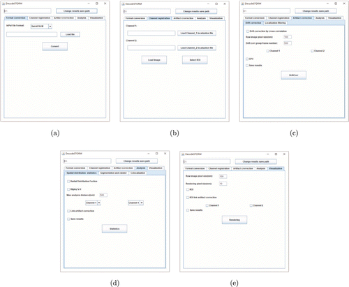
Fig. 1. The modules in DecodeSTORM. (a) Format conversion module, which converts localization table obtained from several typical localization software into the format used in DecodeSTORM. (b) Channel registration module, which is used to import data and select ROI for further analysis. (c) Artifact correction module, which removes artifacts from SMLM data. (d) Quantitative analysis module, which extracts photophysical/biological information from SMLM data. (e) Visualization module, which uses a localization table to generate a super-resolution image.
| Software | Platform | Multichannel | GUI | Drift Correction | Filtering | Visualization | Spatial Statistic | Cluster/Segmentation | Colocalization |
|---|---|---|---|---|---|---|---|---|---|
| ThunderStorm | ImageJ | − | + | + | + | + | − | − | + |
| PALMsiever | Matlab | − | + | + | + | + | − | DBSCAN | − |
| SR-Tesseler | Standalone | − | + | − | + | + | − | Voronoi | − |
| LAMA | Standalone | + | + | − | − | − | + | DBSCAN | + |
| Clus-Doc | Matlab | + | + | − | − | + | + | DBSCAN | + |
| SharpViSu | Matlab | + | + | + | + | + | + | Voronoi | − |
| Grafeo | Matlab | + | + | − | + | + | + | Voronoi | − |
| 3DCluster-ViSu | Matlab | + | + | − | − | + | − | Voronoi | − |
| NanoJ | ImageJ | + | + | + | − | + | − | − | − |
| SMoLR | R | − | − | − | − | + | − | DBSCAN/KDE | − |
| Decode-STORM | ImageJ | + | + | + | + | + | + | DBSCAN/Voronoi | + |
2. Materials and Methods
2.1. Simulated and experimental data
We used the methods reported in Ref. 19 to simulate two SMLM datasets with 40 randomly placed, nonoverlapping clusters in a field of view of 0.2μm∗0.2μm, with an intra-cluster molecular density of 0.01mol/nm2, using one dataset as the ground truth [Fig. 2(a)]. We then added artifacts to the ground truth dataset (see Table 2 for the addition method) to obtain four groups of simulated artifact datasets [Figs. 2(b)–2(e)], with five sets of randomly generated data within each group. In the artifact dataset, the probabilities of isolated localization and imprecise localization were obtained from experimental calculations, and the probabilities of repeated localization from the same fluorophore and repeated localization in the same frame and the amount of drift were set according to the previously reported literature.31,32,33
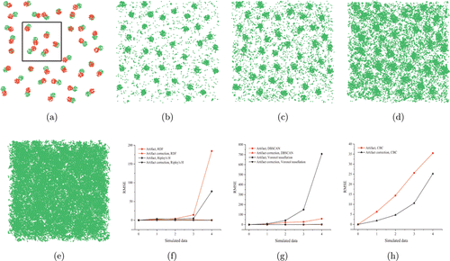
Fig. 2. Analysis of artifacts affecting quantitative analysis of SMLM data. (a) Scatterplot of a simulated data (channel 1: green, channel 2: red). Data in the black box were used in DBSCAN, Voronoi, and CBC analysis. (b)–(e) Scatter plots of the four groups of artifact data mentioned in Table 2. (f)–(h) Comparison of root mean square error of various quantitative analysis results before and after artifact correction.
| Isolated localization (% of the cluster density) | Repeated localization from the same fluorophore (% of the localizations) | Repeated localization in the same frame (Error rate) | Imprecise localization (% of the localizations) | The maximum amount of drift | |
|---|---|---|---|---|---|
| 1 | 2.5% | 12.5% | 6.25% | 0.5% | x:25, y:25 |
| 2 | 5% | 25% | 12.5% | 1% | x:50, y:50 |
| 3 | 10% | 50% | 25% | 2% | x:100, y:100 |
| 4 | 20% | 90% | 50% | 4% | x:200, y:200 |
We downloaded the raw single molecule images of nuclear pore complex (NPC) from the SRM hub (https://srm.epfl.ch/), and performed image processing using QC-STORM to obtain the localization data. The two-color SMLM data were downloaded from the Github repository (https://github.com/PRNicovich/ClusDoC), which was provided by Pageon et al. for testing their Clus-DOC algorithm.21,34 The two-color SMLM data were from T-cell receptor (TCR, green channel) and phosphorylated TCR (pTCR, red channel), in activated Jurkat cells, respectively.
2.2. Artifact correction methods
During an SMLM experiment, thousands of diffraction-limited raw images are acquired, which are further used to obtain the precise locations of millions of fluorescent molecules. Because this imaging process is typically in the order of minutes, several experimental factors, such as temperature changes and mechanical shocks, will make sample drift almost unavoidable, thus resulting in artifacts. Therefore, drift correction is usually required in SMLM. DecodeSTORM provides a widely-used method called redundant cross-correlation (RCC) for drift correction. The RCC method is based on localization events, and has been proven to have good performance.9,35
In the filtering sub-module, DecodeSTORM can filter out four types of false positive localizations caused by different reasons (see below and the user’s guide).
| (1) | Imprecise localization. Localization precision is the estimated error of the localization coordinates, which can be appropriated given as σx,y=s/√N, where s represents the width of point spread function (PSF) and N represents the total number of photons collected from a fluorescent molecule. A larger localization precision value indicates a poorer localization performance, and may deteriorate the final super-resolution image. DecodeSTORM uses a threshold to remove imprecise localization, that is, any localizations with a localization precision value larger than this threshold are removed. | ||||
| (2) | Isolated localization [Fig. 3(a)]. Isolated localization usually comes from autofluorescence and out-of-focus fluorescence. Imaging artifacts caused by isolated localization are evident and usually considered as noise. DecodeSTORM removes isolated localization using a density filtering method, which includes two parameters: (1) The radius r, which determines the size of the area for searching nearest neighbor localization events; (2) the standard deviation (stdev), which determines the minimum number of localization events within the radius. For an area of radius r centered at any localization, when the number of localization events is less than the minimum number threshold, this localization is considered as an isolated localization and would be removed. | ||||
| (3) | Repeated localization in the same frame [Fig. 3(b)]. High-density emitters in a single image frame need to be localized using a proper multiple-emitter localization algorithm. If different ROIs contain data from the same fluorescence spots, this multiple-emitter localization algorithm may misidentify one localization as multiple localizations, and these repeated localizations from the same molecule will appear in the same frame.36 Note that imaging artifacts caused by repeated localization are not easily detected. To remove repeated localization in the same frame, DecodeSTORM uses a distance threshold. Specifically, if the distance between two localizations is less than the distance threshold, the localizations are identified as repeated, and the localization with a larger localization precision value is removed. | ||||
| (4) | Repeated localization from the same fluorophore [Fig. 3(c)]. A single fluorescence molecule may blink many times before bleached, which causes fluorescence signal from the same molecules reappear in subsequent frames. This phenomenon would result in multiple localizations from the same molecule, and thus causes imaging artifacts.16 For repeated localization from the same fluorophore, DecodeSTORM requires users to first set the maximum allowable distance among reappeared localizations, and the number of frames required to merge recurring localizations. Then, in the current frame and a certain number of frames afterwards, the localizations whose inter-localization distance is within the maximum allowed distance are found, identified to be originated from the same molecule, and merged (the localization with the best localization accuracy is selected). | ||||
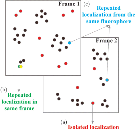
Fig. 3. Imaging artifacts in SMLM. (a) Isolated localization. (b) Repeated localization in the same frame. (c) Repeated localization from the same fluorophore.
2.3. Quantitative analysis methods
G(r) is a probability density function.37 In G(r), a circle of radius r is drawn with a localization as the center, a ring of width D is continuously drawn outside the circle, and the density ρ inside the ring surface is calculated. Then, the probability of finding another localization in the range from r to (r+D) can be calculated as follows :
CBC can be used to calculate the intermolecular spearman correlation coefficient. A CBC value is assigned to each localization: −1 for anti-colocalization or segregation, 0 for no colocalization, and +1 for perfect colocalization.14
2.4. Development of DecodeSTORM
ImageJ39 has become an invaluable laboratory tool because it is free and easy to install. In the past few years, many SMLM software has been reported as ImageJ plug-in. In this paper, we presented DecodeSTORM as an ImageJ plug-in to enable easy software interaction and quantitative data analysis. DecodeSTORM used NetBeans IDE software to develop user-interactive interfaces, and programmed most of the operations, including mainly format conversion, artifact correction, quantization analysis and image rendering, in C++ based on Visual Studio IDE software. We used NVIDIA CUDA to enable a GPU-based computation acceleration for drift correction. To simplify the difficulty in matrix processing and Voronoi Tessellation clustering, DecodeSTORM also used third-party libraries, including calls to the Armadillo and OpenCV libraries.
3. Results and Discussion
3.1. Features of DecodeSTORM
DecodeSTORM was developed to provide a simple and efficient tool for extracting biological information (density, distribution, etc. of biomolecules) for biologists without sufficient computer programming background. Compared to other similar software, DecodeSTORM paid more effort into imaging artifact correction. DecodeSTORM contains five parent modules (Fig. 1): (1) Format conversion, (2) channel registration, (3) artifact correction, (4) quantitative analysis and (5) visualization. The artifact correction module includes two sub-modules (localization filtering and drift correction), and the quantitative analysis module includes three sub-modules (spatial distribution statistics, segmentation and clustering, colocalization). The five parent modules are ordered according to the DecodeSTORM workflow (Fig. 4). We provide an option to save the intermediate results in each module.

Fig. 4. The workflow of DecodeSTORM. In the format conversion module, a localization table generated by several representative localization software (QuickPALM, RapidSTORM, ThunderSTORM, QC-STROM) can be converted to a format suitable for DecodeSTORM. In the Channel registration module, the converted localization table is uploaded and assigned to a proper channel, and then is used to generate a scatter-plot image. Here, two channels are provided for processing two-color SMLM images. With this scatterplot image, users can select a suitable region-of-interest (ROI) for further processing. In the Artifact correction module, localization filtering and drift correction can be applied to the selected ROI, using any combination of the methods in the sub-modules. In the Quantitative analysis module, the ROI with or without artifact correction can be quantitatively analyzed using three different sub-modules including spatial distribution statistics, segmentation and clustering and colocalization. The visualization module is designed to reconstruct a super-resolution image from an ROI or all areas.
3.2. The format conversion module for getting a localization table suitable for DecodeSTORM
DecodeSTORM provides a format conversion module [Fig. 1(a)] for converting a localization table generated by several representative software (QuickPALM,40 RapidSTORM,41 ThunderSTORM,17 QC-STROM42) into a format suitable for DecodeSTORM. The localization table format for DecodeSTORM is a 12-column CSV file listing the following parameters: Peak intensity (photon), x (nm), y (nm), z (nm), PSFSigmaX (nm), PSFSigmaY (nm), Total intensity (photon), background (photon), SNR (peak to background e-), Localization precision X (nm), Localization precision Y(nm), frame. If the raw localization table does not have some of the above parameters, these parameters will be set to 0 in the converted localization table.
3.3. The channel registration module for data import and ROI selection
In the channel registration module, DecodeSTORM provides two channels for importing two-color SMLM data: Channel 1 for green and Channel 2 for red. For single-color SMLM data, users can use either channel, but should remember to select the right channel containing data for subsequent data processing and analysis. Clicking the “Load Image” button will generate a scatterplot of the data. Then, users can select an ROI for artifact correction and/or quantitative analysis. More information can be found in the user’s guide.
3.4. The artifact correction module for removing artifacts
Artifacts are usually generated in SMLM experiments due to various reasons, including but not limited to sample drift and imprecise localization. These artifacts will reduce the image quality and the accuracy of data analysis, and thus should be corrected before quantitative analysis.16 DecodeSTORM provides an artifact correction module [Fig. 1(c)], which includes two sub-modules: Drift correction and localization filtering. Alternatively, if the SMLM data do not require artifact correction, users can skip this step and directly conduct quantitative analysis.
When using drift correction, a pop-up box with correction information will appear. In addition, we provide the option for GPU acceleration (see user’s guide). Users can use any of the localization filtering methods individually or in combination. After clicking the “Filtering” button, a scatter plot for the selected ROI will be generated, which allows the user to compare the scatter-plot images before and after filtering. During the drift correction and localization filtering steps, users are recommended to save the results, before moving to the next step. The results are then saved as CSV files. However, if users do not choose to save the results, the subsequent quantitative analysis will still process the data after artifact correction because the results have been already loaded into the memory.
3.5. The quantitative analysis module for extracting biological information from SMLM data
The quantitative analysis module [Fig. 1(d)] includes three sub-modules, where the raw SMLM data or artifact-corrected SMLM data can be quantitatively analyzed to extract biological information. The first sub-module is called spatial distribution statistics, which is used to extract the distribution information of biological macromolecules, such as the degree of clustering, the radius of clusters, etc. DecodeSTORM allows users to analyze not only self-clustering, but also co-clustering for two-color SMLM data. When users choose G(r) and/or H(r), the parameters need to be set. After pressing the “Statistics Analysis” button, a function graph of G(r) and/or H(r) will be generated. The maximum values of the function and its radius r and cluster size are displayed in the upper right corner. We recommend that users choose to press the button “save results” before moving to the next steps, so that the function value and the corresponding radius r are saved in a CSV file. For the results from G(r) and H(r) calculation, a curve indicates that the SMLM data contain clusters. And, a high peak in the curve means a high degree of clustering. If a line with multiple peaks is produced from G(r) calculation, the ROI may contain multiple clusters with regular spacing and size. Here, the peak width represents the average radius of the clusters, and the distance between the peaks represents the inter-cluster distance. For the results from H(r) calculation, the larger the average size of the cluster, the larger the radius of the peak would be. If a line (x=0) is generated, there are no clusters.
The second sub-module is segmentation and clustering. Include DBSCAN and Voronoi Tessellation, which are used to extract the distribution, number and density of biomolecules, and can be presented as clustering map and Voronoi diagrams. For DBSCAN, after setting the parameters and pressing the “Cluster” button, a clustering map will be generated with different colors representing different clusters. Voronoi Tessellation is adaptive and can be used to directly generate Voronoi diagrams characterizing the molecular density information, where a higher molecular density results in a smaller area in the Voronoi cell.19 When using the above clustering methods, a text box is appeared to show the number and density of clusters.
The third sub-module is colocalization, DecodeSTORM provides a CBC method to study protein interactions.14 A CBC value is assigned to each localization: −1 means anti-colocalization, 0 means no colocalization and 1 means perfect colocalization, respectively. After setting the parameters and pressing the “colocalization” button, a histogram of CBC values will be generated. If users choose to save the results, the percentage of localizations larger than a predetermined colocalization threshold will be saved into a CSV file. More values greater than zero in the histogram indicate a higher degree of colocalization between the two biomolecules and thus stronger interactions. It should be noted that users can choose to use the SMLM data before or after artifact correction for quantitative analysis, and the methods in each sub-module can be used individually or in combination.
3.6. The visualization module for reconstructing super-resolution images
After the SMLM data are imported into a suitable channel, users can apply the visualization module [Fig. 1(e)] to reconstruct a super-resolution image via Gaussian rendering. Here, a Gaussian function is used to approximate the PSF from each localization. In the function, the width of the standard deviation is given by the localization precision, and the peak intensity is given by the fitted peak intensity of the fluorescent spot.30 The visualization module applies to either original SMLM data or artifact-corrected data.
3.7. Validation on simulated data
To verify that the artifact correction provided in DecodeSTORM enhances the accuracy of the quantitative analysis, we used simulated data to perform quantitative analysis on SMLM data before and after artifact correction. We simulated two SMLM datasets, and one of which was used as the ground truth. Four datasets with artifacts were obtained by adding simulated artifacts to the ground truth.
For each case, we compared the quantitative analysis results before and after artifact correction by calculating the root mean square error, where segmentation and clustering, and colocalization are applied to the ROI. Spatial distribution statistical functions are used to calculate cluster sizes, and they are sensitive to large-scale heterogeneity (e.g., inside and outside the cell) and repeated localization from the same fluorophore.37 DBSCAN and Voronoi tessellation are used to calculate the density of clusters, where artifacts may be identified as clusters or cause several clusters to be identified as one. When calculating the percentage of colocalized molecules using CBC, artifacts may be recognized as colocalized molecules, but the percentage of colocalized molecules usually decreases due to an increase in the number of localizations within the channel. The existence of artifacts directly reduces the accuracy of quantitative analysis, and the more the artifacts are present, the more the quantitative analysis is affected. After artifact correction, the RMSE is found to be reduced significantly, which improves the accuracy of the quantitative analysis. A suitable artifact correction brings the RMSE of both the calculated cluster size and density close to 0 [Figs. 2(f) and 2(g)]. However, some errors still exist in the calculation of the percentage of colocalized molecules after artifact correction due to the strong dependence of the CBC calculation on interdot relationships [Fig. 2(h)].
3.8. Validation of experimental data
To verify the usefulness of DecodeSTORM in the experimental data, we first performed a quantitative analysis of the raw and artifact-corrected data of ROI in the NPC dataset using DecodeSTORM (Fig. 5). We calculated the average diameter of all clusters using H(r). The diameter from the raw data is 130.76924nm and from the artifact-corrected data is 123.07692nm [Figs. 5(d) and 5(e)]. Note that the diameter of the artifact-corrected data is closer to the known size.29,43 Note that G(r) does not apply to our data, and that the cluster size calculated using G(r) is significantly smaller than the true size of the cluster. However, the findings above demonstrate the necessity of G(r) to some extent. For example, Caetano et al. used G(r) to observe that the size of β2-adrenergic receptor cluster after 5min of isoproterenol stimulation was approximately 90nm, which closely matches the reported size of clathrin-coated pits.38 Cluster densities of ROI were calculated using DBSCAN and Voronoi tessellation, and the densities of the artifact-corrected data were almost identical to the previous values43: 7.407μm−2 from DBSCAN, and 6.172μm−2 from Voronoi tessellation [Figs. 5(h) and 5(i)]. However, the densities calculated from the raw data (without artifact correction) deviated significantly from the previously reported values: 45.674μm−2 from DBSCAN, and 104.9383μm−2 from Voronoi tessellation [Figs. 5(f) and 5(g)].
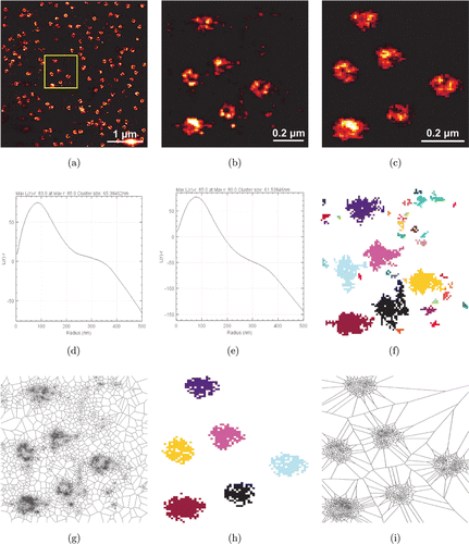
Fig. 5. Size and density analysis of NPC using DecodeSTORM. (a) A reconstructed super-resolution image obtained by Gaussian rendering of NPC localization data using DecodeSTORM. (b) A reconstructed super-resolution image of the data in the yellow box in (a), where the data were used for subsequent analysis. (c) A reconstructed super-resolution image of the data in (b) after artifact correction. (d) and (e) H (r) of all clusters before and after artifact correction. (f) and (g) DBSCAN clustering map (f) and Voronoi diagram (g) of ROI (yellow box in a) before artifact correction. (h) and (i) DBSCAN clustering map (h) and Voronoi diagram (i) of ROI (yellow box in a) after artifact correction.
Next, we applied DecodeSTORM to the two-color SMLM data of TCR and pTCR and analyzed the degree of colocalization in their ROI regions using CBC. Note that the pTCR should be highly colocalized with the TCR.21 We found that the percentage of colocalized pTCR molecules for the data without artifact correction is less than 50% (48.77%), while the percentage of colocalized pTCR molecules after artifact correction is 58.97%, showing a higher degree of colocalization after artifact correction [Figs. 6(c) and 6(d)].
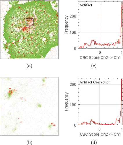
Fig. 6. Colocalization analysis of TCR and pTCR using DecodeSTORM. (a) Scatterplot of TCR and pTCR. (b) An enlarged image from the black region in (a), where the data were used for colocalization analysis. (c) Histogram of TCR→pTCR colocalization values before artifact correction. (d) Histogram of TCR→pTCR colocalization values after artifact correction.
DecodeSTORM processed the ROI data from NPC [Figs. 5(a) and 5(b)], where the artifact correction took about 4s, G(r), H(r), and DBSCAN took less than 1s. Voronoi took 28min, but these data take about 1min to perform Voronoi in Cluster ViSu.29 In fact, Voronoi is computationally huge. ClusterViSu uses CPU Parallel to accelerate Voronoi, which is merely encapsulated in DecodeSTORM without acceleration. We will improve Voronoi speed in a subsequent release. DecodeSTORM took about 10s when calculating the colocalization of the two-color data (data in ROI) after artifact correction [Figs. 6(a) and 6(b)]. The evaluations were performed under a commercial PC equipped with 8-core CPU (Intel Core i7-9700), 32GB memory, and a graphics card (NVIDIA GeForce RTX 2070s, with 2560 CUDA cores and 8GB memory).
4. Conclusions
DecodeSTORM is an interactive and modular ImageJ plug-in that implements various methods for quantitative analysis of SMLM data. The integration of artifact correction methods further improves the power of this new plug-in, while the availability of visualization helps users to observe directly super-resolution images. DecodeSTORM has a good potential to become an important tool for biologists who are trying to use SMLM in answering important biological questions, since DecodeSTORM makes it easy to freely combine different SMLM data analysis methods. If the users have some computer programming experience, they can also integrate DecodeSTORM into their own data acquisition software under a popular platform called Micro-Manager. In summary, DecodeSTORM is dedicated to providing biologists with a convenient and reliable tool for SMLM data analysis. The primary goal for this plug-in is to enable widespread use of SMLM and thus bring more opportunities for the development of SMLM data analysis tools.
Acknowledgments
We thank the authors in Refs. 21 and 34 for providing datasets, which were downloaded at https://github.com/PRNicovich/ClusDoC. This work is supported by the National Natural Science Foundation of China (82160345), Key research and development project of Hainan province (ZDYF2021GXJS017), Key Science and Technology Plan Project of Haikou (2021-016), the Start-up Fund from Hainan University (KYQD(ZR)-20022 and KYQD(ZR)-20077) and the Student Innovation and Entrepreneurship Project of Biomedical Engineering School, Hainan University (BMECF2D2021001).
Conficts of Interest
The authors have no conficts of interest to declare.

